In Excel, to find the maximum, minimum and average value in the range and return the corresponding value from another range, use the VLOOKUP formula with the AVERAGE, MAX and MIN functions.
VLOOKUP looks up the value in the left-most column of the source data and returns the corresponding value from the right column.
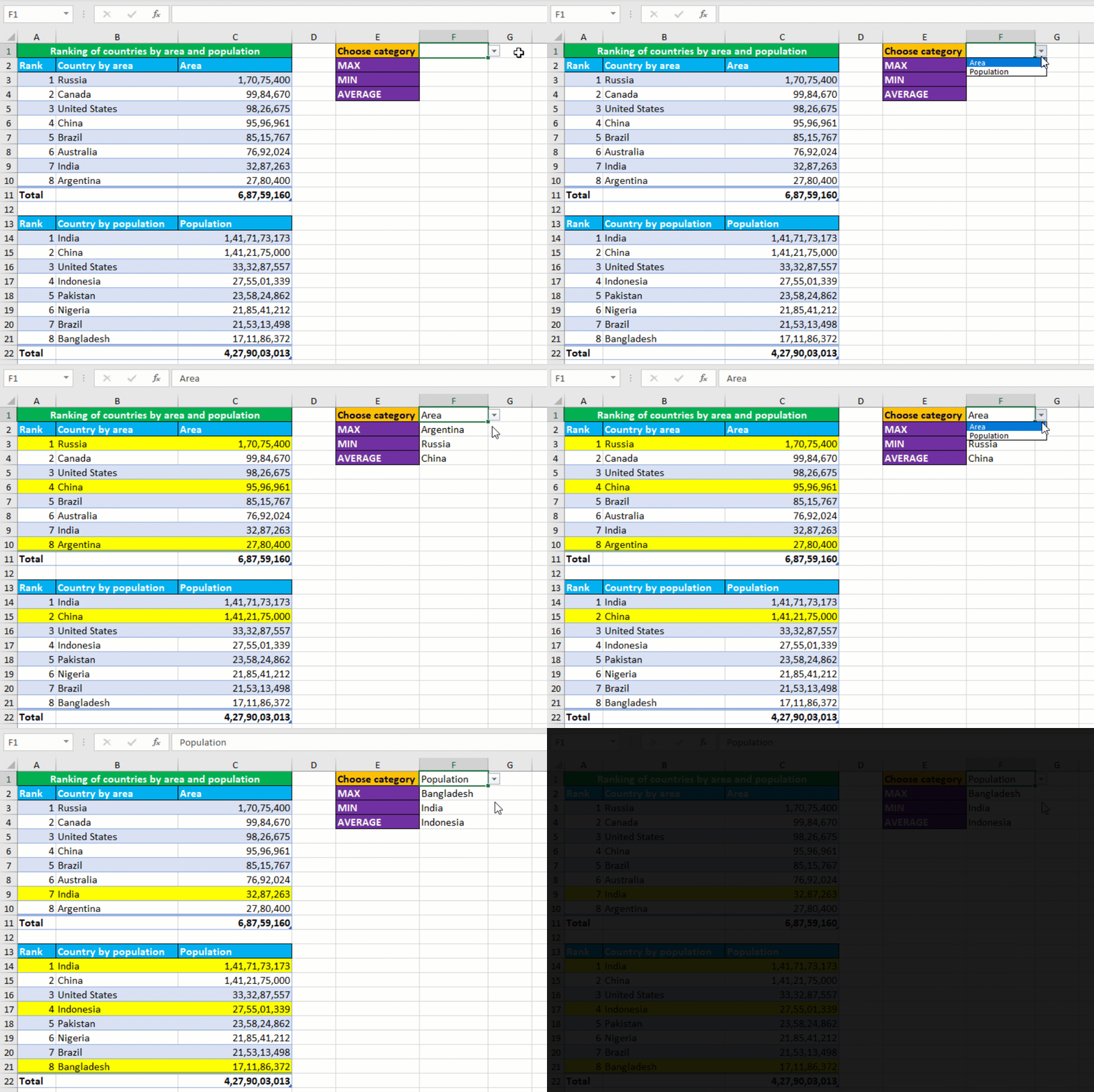
I have the following dataset. Now I want that when the user makes a selection from the dropdown (Area, Population) in F1, the program will calculate the maximum, minimum and average value in column A (Rank) depending on the selection and return the corresponding value from column B, like shown below:

To accomplish the task, I perform the following steps:
Convert both the source data into an Excel table separately. To do so, select the source data range (including the headers), go to the Insert tab and click on the Table button.
Create named ranges separately for both the tables. From the first table, select column A and B data and name it as area in the name box. Do the same for the second table and name it as population.
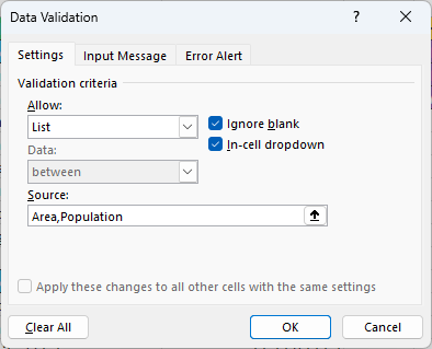
Use data validation to create category dropdown list in F1, listing area and population ranges. To do so, go to Data > Data Validation > Allow: List > Source: Area,Population

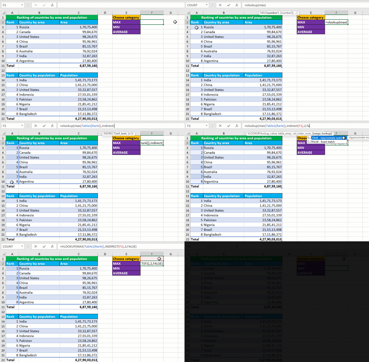
To find the maximum value in column A depending on the selection from F1 and return the corresponding value from column B, construct the following formula in F2, like shown below:
=IFERROR(VLOOKUP(MAX(Table1[Rank]),INDIRECT(F1),2,FALSE),"")

To find the minimum value in column A depending on the selection from F1 and return the corresponding value from column B, construct the following formula in F3, like shown below:
=IFERROR(VLOOKUP(MIN(Table1[Rank]),INDIRECT(F1),2,FALSE),"")

To find the average value in column A depending on the selection from F1 and return the corresponding value from column B, construct the following formula in F4, like shown below:
=IFERROR(VLOOKUP(AVERAGE(Table1[Rank]),INDIRECT(F1),2,TRUE),"")

To replace the REF! error with an empty string "", nest all the formulas in the IFERROR function.
Your dropdown VLOOKUP with AVERAGE, MAX, MIN calculator is ready! I hope this post helped you.


