Here, we will learn how to use the Excel logical functions: IF, AND, OR, NOT, TRUE and FALSE functions. Later, we will also learn how to construct the IF AND OR statement using the ISBLANK function.
IF function
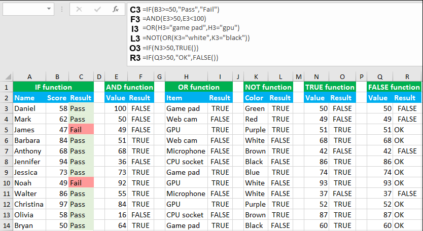
The Excel IF function tests the condition and returns a value if the condition evaluates to TRUE or another value if FALSE. The formula in C3, copied down, is:
=IF(B3>=50,"Pass","Fail")
The formula reads "return Pass for scores greater than or equal to 50 and Fail for scores less than 50". As the formula is copied down, the formula returns "Pass" if the corresponding cell in column B contains a number greater than or equal to 50 and "Fail" if the number is less than 50.
AND function
The Excel AND function checks if the given conditions in a test are TRUE. For example, you can test if the number in A1 is greater than zero and less than 10, by using =AND(A1>0,A1<10). The formula in F3, copied down, is:
=AND(E3>50,E3<100)
Translated in English, the formula reads "return TRUE for the value that is greater than 50 AND less than 100, FALSE otherwise". As the formula is copied down, the formula returns TRUE if the corresponding cell in column E contains a number greater than 50 and less than 100 and FALSE if the number is less than or equal to 50 or greater than or equal to 100.
OR function
The Excel OR function checks if any given condition in a test is TRUE. It returns FALSE if all the given conditions evaluate to FALSE. For example, to test A1 for either "a" or "b", use =OR(A1="a",A1="b"). The formula in I3, copied down, is:
=OR(H3="game pad",H3="gpu")
Translated in English, the formula reads "return TRUE for the item that is game pad OR gpu, FALSE otherwise". As the formula is copied down, the formula returns TRUE if the corresponding cell in column H contains the items "game pad" or "gpu" and FALSE if it is not "game pad" or "gpu".
NOT function
The Excel NOT function returns the opposite of the given Boolean value. For example, for TRUE, NOT returns FALSE and for FALSE, NOT returns TRUE. The formula in L3, copied down, is:
=NOT(OR(K3="white",K3="black"))
Translated in English, the formula reads "NOT white or black". As the formula is copied down, the formula returns TRUE if the corresponding cell in column K is not "white" or "black" and FALSE if it is "white" or "black".
TRUE function
The Excel TRUE function returns the Boolean value TRUE and it is mainly used with the IF function. For example, to return the value TRUE, use =TRUE(). The formula in O3, copied down, is:
=IF(N3>50,TRUE())
As the formula is copied down, the formula returns TRUE if the corresponding cell in column N contains a number greater than 50 and FALSE if it is less than or equal to 50.
FALSE function
The Excel FALSE function returns the Boolean value FALSE and it is mainly used with the IF function. For example, to return the value FALSE, use =FALSE(). The formula in R3, copied down, is:
=IF(Q3>50,"OK",FALSE())
As the formula is copied down, the formula returns OK if the corresponding cell in column Q contains a number greater than 50 and FALSE if it is less than or equal to 50.
IF AND OR statement using the ISBLANK function
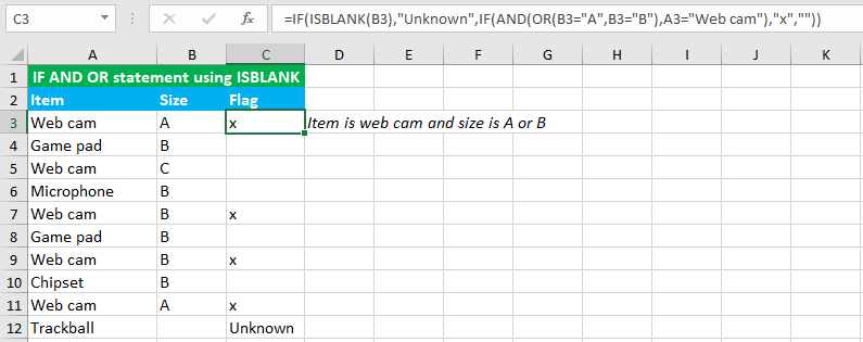
In the example below, the goal is to mark the rows where the item is "Web cam" and the size is "A" or "B". Moreover, if a cell in column B is blank, the corresponding formula should return "Unknown".
To accomplish the task, I use the nested IF formula in C3 using ISBLANK and the IF AND OR statement:
=IF(ISBLANK(B3),"Unknown",IF(AND(OR(B3="A",B3="B"),A3="Web cam"),"x",""))

As the formula is copied down, the formula returns "x" if the corresponding cell in column B contains "A" or "B" and column A contains "Web cam".
You have successfully learnt how to use the Excel logical functions: IF, AND, OR, NOT, TRUE and FALSE functions and how to construct the IF AND OR statement using the ISBLANK function! I hope this post helped you.


