Here, we will learn how to use the Excel information function: ISERROR. Later, we will also learn how to compare data with errors using ISERROR with the IF function.
ISERROR function
The Excel ISERROR function returns TRUE when the given value is an Excel error and FALSE if it is not: The given value to the function must be one of the following Excel errors: #N/A, #VALUE!, #REF!, #DIV/0!, #NUM!, #NAME?, #NULL!, #CALC!, or #SPILL!.
The function takes just one argument, value, that needs to be tested. The return value of the function is always a Boolean value (TRUE or FALSE). Providing an empty string ("") to the function like so: =ISERROR("") returns FALSE as there is no error.
Examples
The formula =ISERROR(#N/A) returns TRUE, as the given value is an error. Similarly, =ISERROR(10/0) returns TRUE as the given formula =10/0 returns the DIV/0! error as division by zero is not possible. The formula =ISERROR(10) returns FALSE, as the given value is not an error.
Comparing data with errors using ISERROR with IF
To compare data with errors, use IFERROR and nest it in the logical_test argument of IF. In the value_if_false argument, use another IF formula.
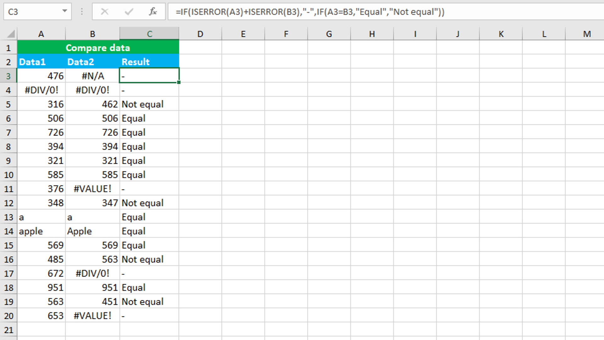
The dataset (shown in the image) contains two data columns: A and B. The goal is to return the dash (-) in the corresponding cell of the column C (Result) if both the cells or one of the cells in columns A and B contain(s) an error. If neither of the cells contains an error, and the value in both the cells is the same, the formula must display the text "Equal", "Not equal" otherwise. The formula in C3, copied down, is:
=IF(ISERROR(A3)+ISERROR(B3),"-",IF(A3=B3,"Equal","Not equal"))
How this formula works
Since A3 contains a number value, =ISERROR(A3) returns FALSE and since B3 is an error value, =ISERROR(B3) returns TRUE. Both FALSE and TRUE values are converted to 0 and 1 respectively. Both are added: 0+1, that gives 1. The condition evaluates to TRUE and the formula returns the dash (-) for TRUE. When the condition evaluates to FALSE, the second IF formula is tested. When the value in A3 is equal to B3, and is not an error, the formula will return the text "Equal". When the value in A3 is not equal to B3, and is not an error, the formula will return the text "Not equal".
You have successfully learnt how to use the Excel information function: ISERROR, and how to compare data with errors using ISERROR with the IF function! I hope this post helped you.