Here, we will learn how to use the Excel text functions: UNICHAR and UNICODE. Later, we will also learn how to generate circled numbers/alphabets using UNICHAR with the ROW function.
Excel UNICHAR function
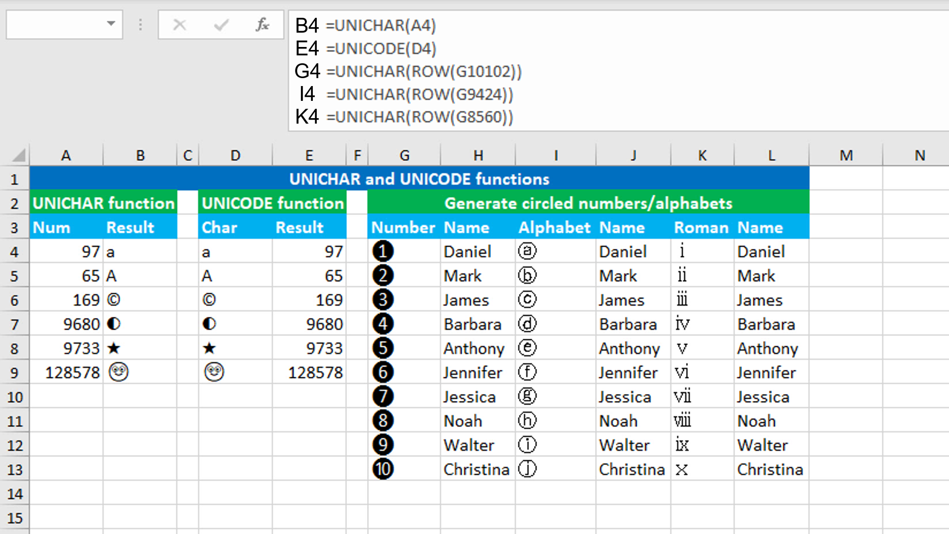
The Excel UNICHAR function returns the Unicode character based on the given Unicode number. For example, to generate the copyright symbol, use the Unicode number 169, like so: =UNICHAR(169). To generate alphabetical series in upper case, use the Unicode numbers from 65 to 90, while to generate in small case, use from 97 to 122. Use the Unicode numbers from 48 to 57 to generate numbers from 0 to 9. The function always returns the result in the text format even if the return value is a numeric value. The formula in B4, copied down, is:
=UNICHAR(A4)
Excel UNICODE function
The Excel UNICODE function returns the Unicode number based on the given Unicode character. For example, with the chess pawn icon in A1, use UNICODE like this: =UNICODE(A1), that returns the Unicode number 9823. The formula in E4, copied down, is:
=UNICODE(D4)
Generating circled numbers/alphabets using UNICHAR with ROW
To generate circled numbers/alphabets, use UNICHAR and supply the ROW function (returns the row number for a reference) in the number argument of UNICHAR.
The dataset (shown in the image) contains a list of names in columns H, J and L. The goal is to generate sequential numbers in column G for the names in column H, alphabetical series in column I for the names in column J and roman numbers in column K for the names in column L. To accomplish the task, the following three formulas are entered.
The formula in G4, copied down, is:
=UNICHAR(ROW(G10102))
The formula in I4, copied down, is:
=UNICHAR(ROW(G9424))
The formula in K4, copied down, is:
=UNICHAR(ROW(G8560))
How these formulas work
The expression =ROW(G10102) in the G4 formula is evaluated, and returns 10102. This number goes to the number argument of UNICHAR and thus, UNICHAR returns the circled number 1. 10102 is the Unicode number for the circled number 1. The circled number 1 is incremented by 1 for each row and so, UNICHAR returns the circled number 2 for 10103 in the next row, circled number 3 for 10104 in the third row, and so on.
Similarly, for the formula in I4, the expression =ROW(G9424) is evaluated, and returns 9424. This number goes to the number argument of UNICHAR and thus, UNICHAR returns the circled letter "a". 9424 is the Unicode number for the circled letter "a". The circled letter "a" is incremented by 1 for each row and so, UNICHAR returns the circled letter "b" for 9425 in the next row, circled letter "c" for 9426 in the third row, and so on.
For the third formula in K4, the expression =ROW(G8560) is evaluated, and returns 8560. This number goes to the number argument of UNICHAR and thus, UNICHAR returns the circled roman number "i". 8560 is the Unicode number for the circled roman number "i". The circled roman number "i" is incremented by 1 for each row and so, UNICHAR returns the circled roman number "ii" for 8561 in the next row, circled roman number "iii" for 8562 in the third row, and so on.
You have successfully learnt how to use the Excel text functions: UNICHAR and UNICODE. You have also learnt how to generate circled numbers/alphabets using UNICHAR with ROW! I hope this post helped you.