Here, we will learn how to use the Excel dynamic array function: HSTACK. Later, we will also learn how to combine and sort unique arrays horizontally using HSTACK and the IFNA, SORT and UNIQUE functions.
HSTACK function
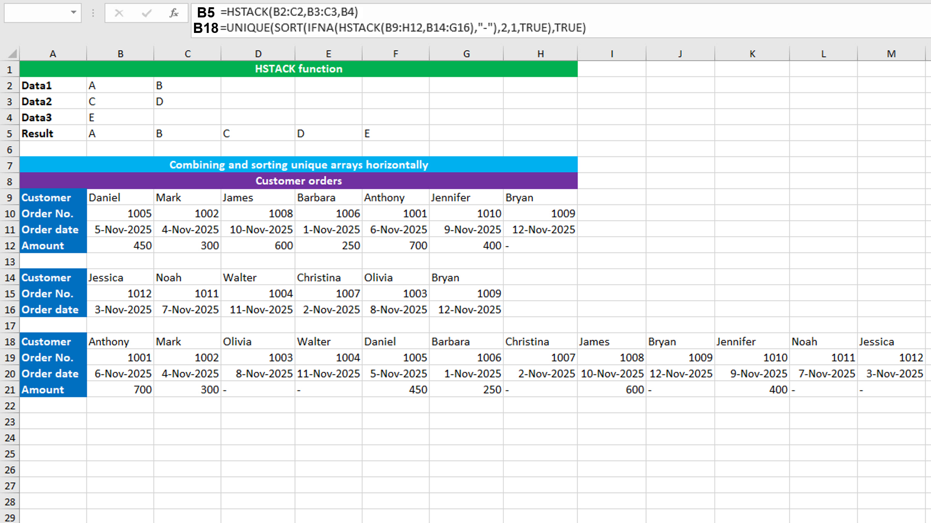
The Excel HSTACK function combines arrays horizontally into a single array, appending each array to the right of the previous array. The result of the function is always a single horizontal array that spills into the multiple cells automatically.
HSTACK takes array arguments: array1, [array2],... The first required argument array1 will take the range to combine. Thereafter, it will take the subsequent optional additional ranges to be combined horizontally.
Let's understand a basic example. You have three sets of data (shown in the image) as "Data1", "Data2" and "Data3". You create a helper column "Result" in row 5 to combine all these three sets of data horizontally. Use HSTACK like this: =HSTACK(B2:C2,B3:C3,B4).
Combining and sorting unique arrays horizontally using HSTACK with IFNA, SORT and UNIQUE
To combine and sort unique arrays horizontally, use the formula based on HSTACK, IFNA, SORT and UNIQUE functions.
The dataset (shown in the image) contains the data about customer orders that is separated into two ranges B9:H12 and B14:G16. The goal is to combine these two ranges horizontally using HSTACK. However, note that both the ranges are of different size and combining both of them will force HSTACK to expand the smaller array to match the size with the larger array and will fill the new cells with the #N/A error. To remove this error, nest the HSTACK formula inside the IFNA function. Furthermore, we want the combined range to be sorted by the second row "Order No." in ascending order and want only unique records.
The formula in B18 is:
=UNIQUE(SORT(IFNA(HSTACK(B9:H12,B14:G16),"-"),2,1,TRUE),TRUE)
How this formula works
HSTACK combines both the ranges B9:H12 and B14:G16 horizontally into a single array, spilling the results into the multiple cells automatically in the range B18:M21. HSTACK expands the smaller range to match the size with the larger range and fills the new cells with the #N/A error. IFNA is configured to replace the #N/A error with the dash "-", like this: IFNA(HSTACK(...),"-"). SORT is configured to sort the result range horizontally by the second row "Order No." in ascending order, like this: SORT((HSTACK(...)),2,1,TRUE). Finally, UNIQUE returns unique records in the result range.
You have successfully learnt how to use the Excel dynamic array function: HSTACK, and how to combine and sort unique arrays horizontally using HSTACK and the IFNA, SORT and UNIQUE functions! I hope this post helped you.