Here, we will learn how to construct the formula based on nested XLOOKUP, SUM and IFERROR.
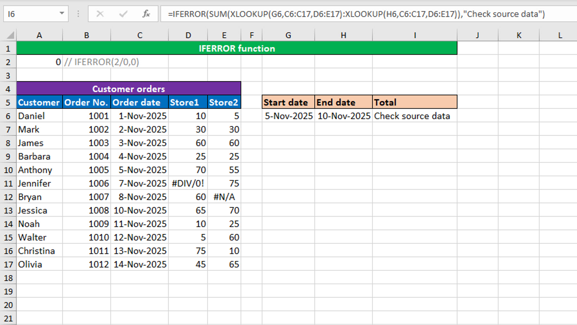
The dataset (shown in the image) contains information about customer orders in two stores. The goal is to sum up the total amount of multiple records by order date.
The formula in I6, is:
=IFERROR(SUM(XLOOKUP(G6,C6:C17,D6:E17):XLOOKUP(H6,C6:C17,D6:E17)),"Check source data")
How this formula works
Both the XLOOKUP formulas are joined with the colon range operator to create a range dynamically. The first XLOOKUP formula retrieves the values 70 and 55 dynamically, like this: =D10:E10. The second XLOOKUP formula retrieves the values 65 and 70 dynamically, like this: =D13:E13. Both these ranges goes to SUM, like this: =SUM(D10:E10:D13:E13). Since the spill range D10:E10:D13:E13 contains the first error #DIV/0!, SUM returns the #DIV/0! error. This error goes to IFERROR that traps it and returns the custom message "Check source data" as the final output.
Note that IFERROR traps any kind of Excel error. If you misspell a function's name, IFERROR will trap the #NAME? error and it would become difficult to solve the issue. In such a case, it becomes sense to use the IFNA function that traps only the #N/A error.
Tip: You can use the Evaluate Formula feature (Formulas > Evaluate formula) to watch how the formula works.
You have successfully learnt how to construct the formula based on nested XLOOKUP, SUM and IFERROR! I hope this post helped you.