Here, we will learn how to use the Excel lookup and reference functions: CHOOSE, INDEX, INDIRECT, MATCH and OFFSET.
CHOOSE function
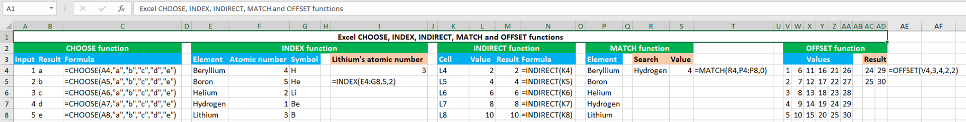
The Excel CHOOSE function returns a value from a list using the given position. For example, =CHOOSE(3,"a","b","c","d","e") returns "c", since "c" is at the third position is the list. The function can be found in all the versions of Excel. CHOOSE takes the arguments like this: (index_num, value1, [value2],…), of which index_num and value1 are required. Index_num accepts the numeric position of the value to return. Value1 accepts the first value from which to choose. Thereafter, the function accepts the subsequent optional value arguments. The formula in B4, copied down, is:
=CHOOSE(A4,"a","b","c","d","e")
INDEX function
The Excel INDEX function returns the value at the given location in the given array or range. In the example shown, the goal is to get the atomic number of the element "Lithium". INDEX returns the value 3, since "Lithium" is in the fifth row and the required atomic number is in the second column in the range E4:G8. Alternatively, you can use this formula: =INDEX(F4:F8,5). The function can be found in all the versions of Excel. INDEX takes the arguments like this: (array, row_num, [col_num]), of which array and row_num are required. Array accepts the array or range from which to return the value. Row_num accepts the row number in the array or range from which to return the value. Col_num accepts the column number in the array or range from which to return the value. The formula in I4, is:
=INDEX(E4:G8,5,2)
INDIRECT function
The Excel INDIRECT function returns a valid cell reference from the given text string. For example, with the value 1000 in A1, you can use INDIRECT like this: =INDIRECT("A1"), that returns the reference to A1, that is 1000. The function can be found in all the versions of Excel. INDIRECT takes the arguments like this: (ref_text, [a1]), of which ref_text is required. Ref_text accepts the reference supplied as text. A1 controls the reference style. It is a Boolean argument that accepts either TRUE to use A1 style reference or FALSE to use R1C1 style reference. If the argument is skipped, it defaults to TRUE. The formula in M4, copied down, is:
=INDIRECT(K4)
MATCH function
The Excel MATCH function searches for the given item in the given array or range, and then returns the numeric position of that item in that array or range. In the example shown, the goal is to get the numeric position of the element "Hydrogen" in the range K4:K8. MATCH returns the value 4, since "Hydrogen" is at the fourth position in the range K4:K8. The function can be found in all the versions of Excel. MATCH takes the arguments like this: (lookup_value, lookup_array, [match_type]), of which lookup_value and lookup_array are required. Lookup_value accepts the value you want to find. Lookup_array accepts the array or range to search in. Match_type controls the match type. It accepts 1 for exact or next smallest, 0 for an exact match or -1 for exact or next largest. The formula in S4, is:
=MATCH(R4,P4:P8,0)
OFFSET function
The Excel OFFSET function returns a reference to a range that is the given number of rows and columns from a cell or a range. For example, to reference I4 starting at A1, use OFFSET like this: =OFFSET(A1,3,8). The formula moves 3 rows below and 8 columns to the right of A1, and therefore references I4. The function can be found in all the versions of Excel. OFFSET takes the arguments like this: (reference, rows, cols, [height], [width]), of which reference, rows and cols are required. Reference accepts the starting point, supplied as a cell reference. Rows accepts the number of rows to offset below the starting point. Cols accepts the number of columns to offset to the right of the starting point. Height accepts the number of rows to return. Width accepts the number of columns to return. The formula in AC4, is:
=OFFSET(V4,3,4,2,2)
The formula moves 3 rows below, 4 columns to the right of V4, in a 2-row by 2-column range and therefore, references the range Z7:AA8.
You have successfully learnt how to use the Excel lookup and reference functions: CHOOSE, INDEX, INDIRECT, MATCH and OFFSET.