Here, we will learn how to convert horizontal data to vertical using the Excel WRAPCOLS and TOROW functions in one formula.
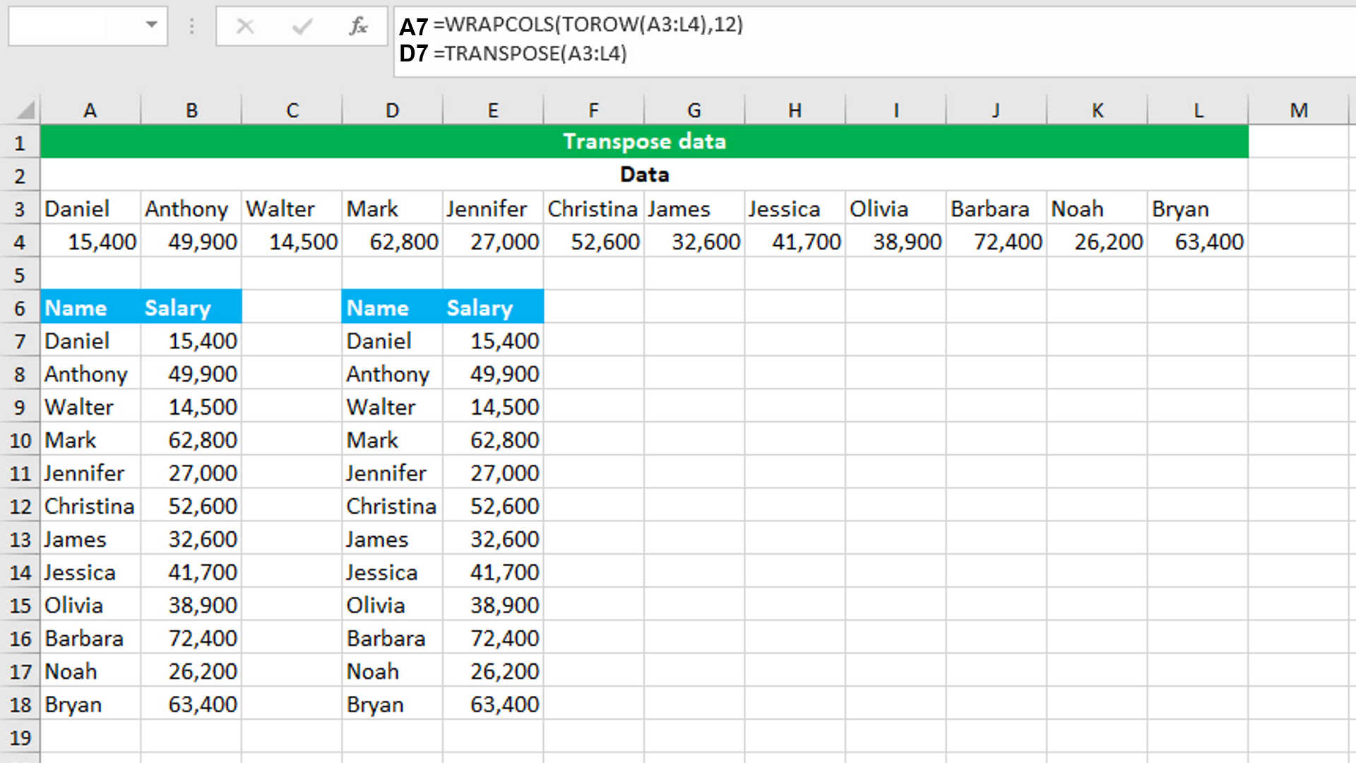
The dataset (shown in the image) containing data about employees and their monthly salaries is arranged horizontally. The goal is to convert the horizontal data into the vertical direction. To accomplish the task, we create the header columns "Name" and "Salary" in the cells A6 and B6 respectively and use the WRAPCOLS and TOROW functions in one formula.
The formula in A7, is:
=WRAPCOLS(TOROW(A3:L4),12)
As soon as I press Enter, the formula spills the results into the multiple cells automatically in the range A7:B18.
How this formula works
TOROW transforms the array A3:L4 into a single row, scanning the values by row and returns the array to WRAPCOLS. WRAPCOLS wraps the array into columns that each contain 12 values. Therefore, we get the horizontal data transformed to vertical data.
Note that the same result can be achieved by using the TRANSPOSE function also. The formula in D7, is:
=TRANSPOSE(A3:L4)
Here, TRANSPOSE flips the horizontal range to the vertical range.
You have successfully learnt how to convert horizontal data to vertical using the Excel WRAPCOLS and TOROW functions in one formula! I hope this post helped you.