Here, we will learn how to use the Excel dynamic array function: DROP. Later, we will also learn how to extract the last n rows using DROP and the ROWS function, that returns the count of rows in the reference.
DROP function
The Excel DROP function returns a subset of the array by removing rows and columns.
DROP takes three arguments: array, rows and cols. The first required argument array, will take the range from which to remove rows and columns. Both rows and cols arguments are optional, but a numeric value is required for at least one. Both accept positive or negative numbers. Positive numbers will remove values from the start of the array; negative numbers will remove values from the end of the array. If no numeric value is provided to rows and cols, both the arguments will take the default value of zero, meaning the formula will return all rows and columns.
Extracting last n rows using DROP and ROWS
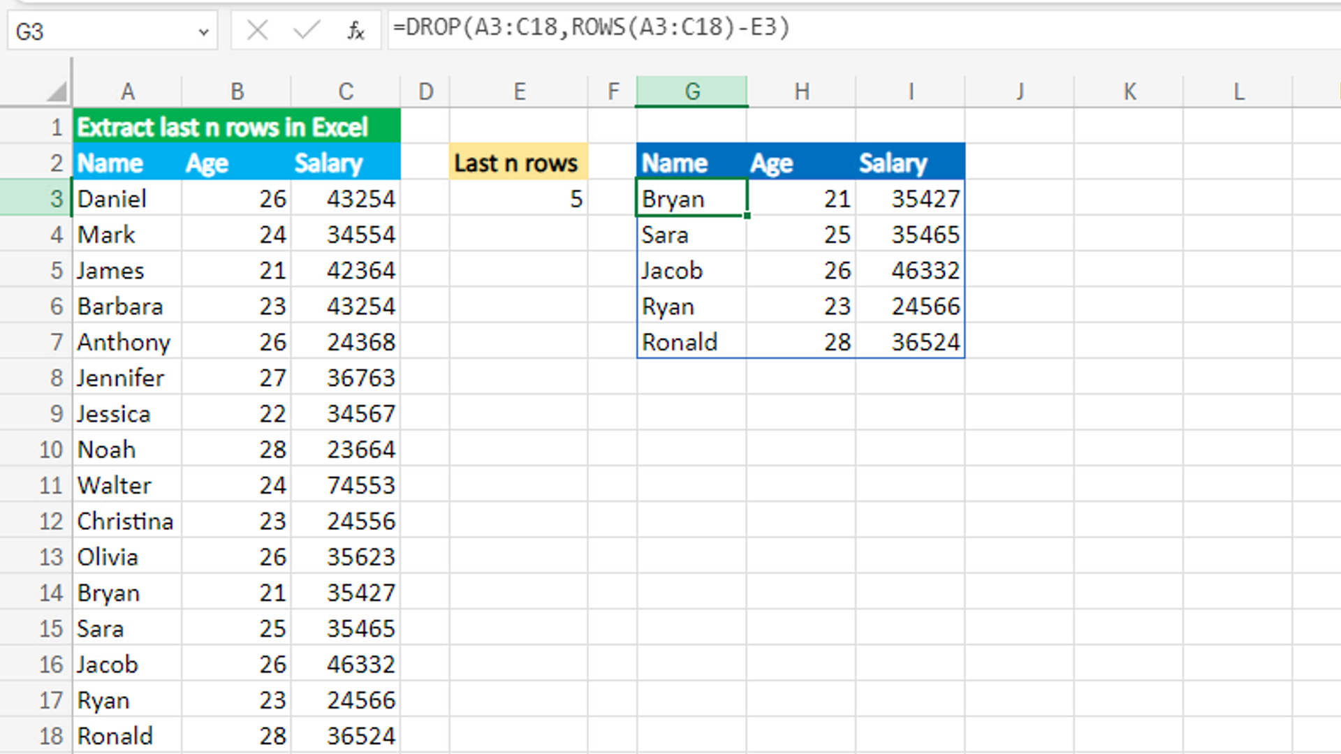
To extract the last n rows from the array, use the DROP formula and nest the ROWS function in the rows argument. My goal is to extract the last 5 rows from the array A3:C18. The formula in G3 is:
=DROP(A3:C18,ROWS(A3:C18)-E3)
Now when I enter the number 5 in E3, the formula in G3 extracts the last 5 rows from the array A3:C18.
As soon as I press Enter, the formula spills the results into the multiple cells automatically in the range G3:I7.
How this formula works
Since there are 16 rows in the array A3:C18, the expression ROWS(A3:C18) returns 16. The value in E3 is 5, so 16-5 equals 11. Since the number 11 is positive, DROP removes 11 rows from the start of the array A3:C18, and returns the remaining rows. Cols defaults to zero, returning all the columns.
You have successfully learnt how to use the Excel dynamic array function: DROP, and how to extract the last n rows! I hope this post helped you.


