In Excel, to return the sum from a set of records that match the criteria selected from the dropdown list, I will use an Excel table, data validation to create dynamic dropdown and the DSUM function.
The following dataset contains the number of chocolates consumed:
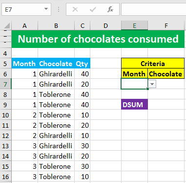
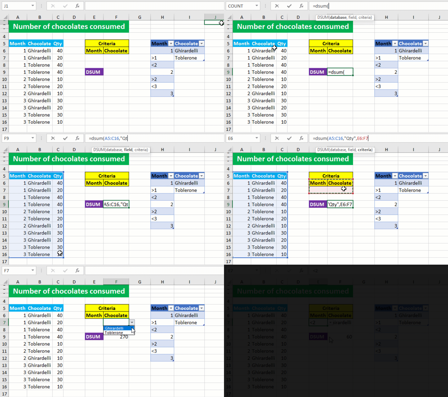
Now I want the program to return the sum of the values in F9 from the field Qty that match the criteria selected from the Month and Chocolate dropdowns in E7 and F7 respectively. To accomplish the task, I perform the following steps:
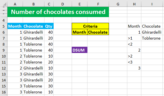
I enter the Month and Chocolate criteria in columns H and I, like so:
I convert the criteria into an Excel table separately, like shown below:
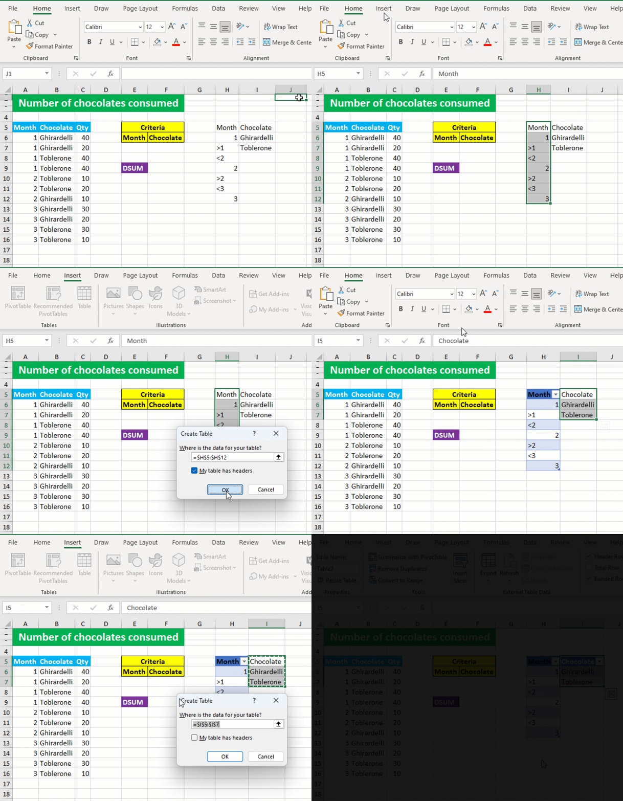
By creating Excel table for both Month and Chocolate, I can create dynamic dropdown list for both.
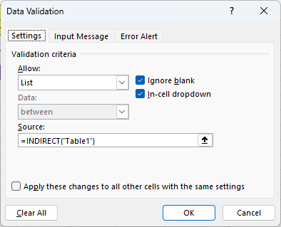
I use data validation to create Month dynamic dropdown list in E7, listing all the Month criteria in Table1, by going to Data > Data Validation > Allow: List > Source: =INDIRECT("Table1")
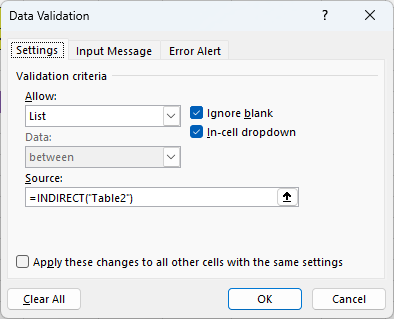
I use data validation to create Chocolate dynamic dropdown list in F7, listing all the Chocolate criteria in Table2, by going to Data > Data Validation > Allow: List > Source: =INDIRECT("Table2")
After all this, I construct my DSUM formula in F9, like shown below:
Your dropdown DSUM formula is ready! I hope this post helped you.


