In Excel, to highlight the matching row based on the selection of the dropdown list and ticking the check box, I will use an Excel table, data validation to create dropdown, checkbox and conditional formatting.
The following dataset contains the number of ice creams consumed. Now I want the program to highlight the matching row only when the user makes a selection of the ice cream from the dropdown list in F6 and ticks the highlight checkbox, like shown below:
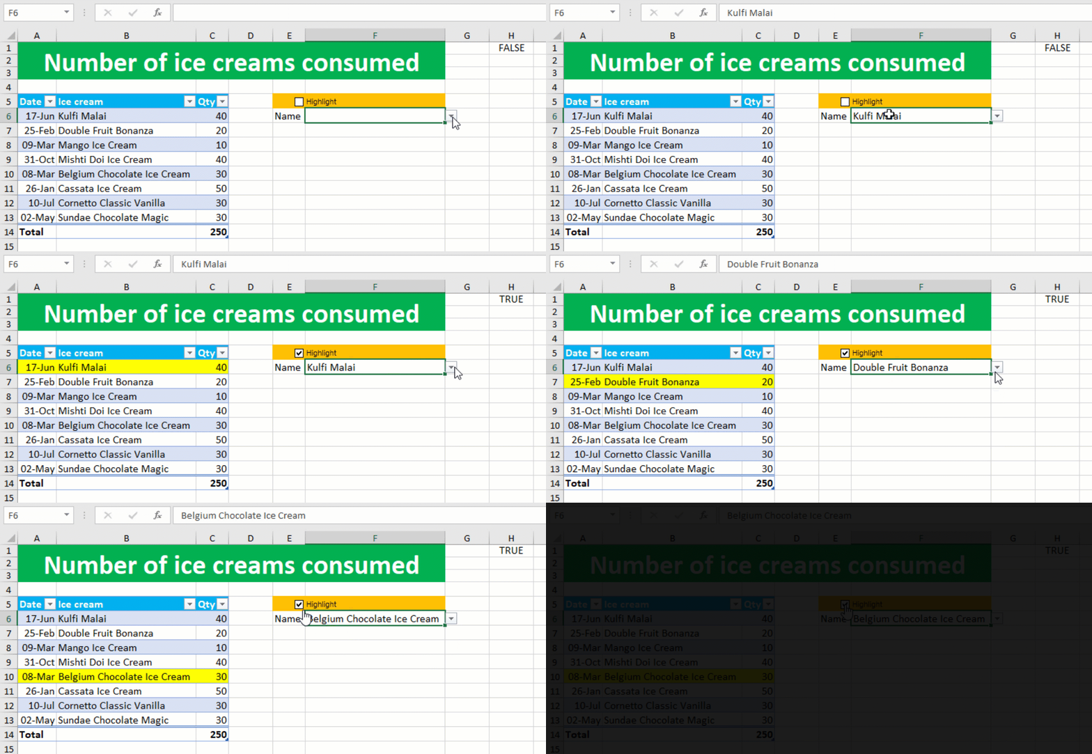
In order to accomplish the task, I perform the following steps:
Convert the source data into an Excel table and name it as data, like shown below:
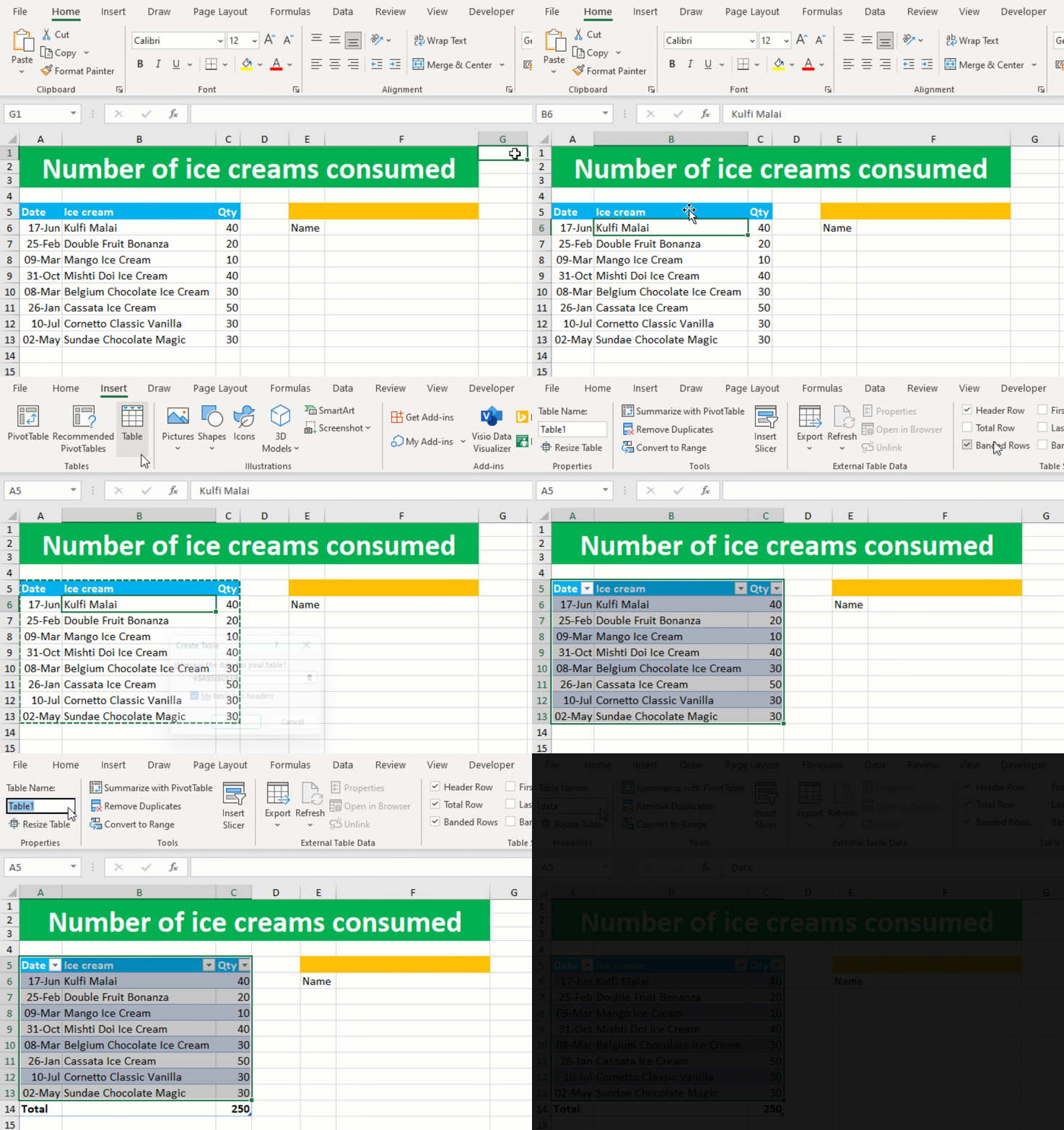
By creating an Excel table, you can create a dynamic dropdown list.
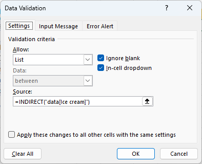
Use data validation to create a dynamic dropdown list in F6, listing all the ice creams in column B, by going to Data > Data Validation > Allow: List > Source: =INDIRECT("data[Ice cream]")
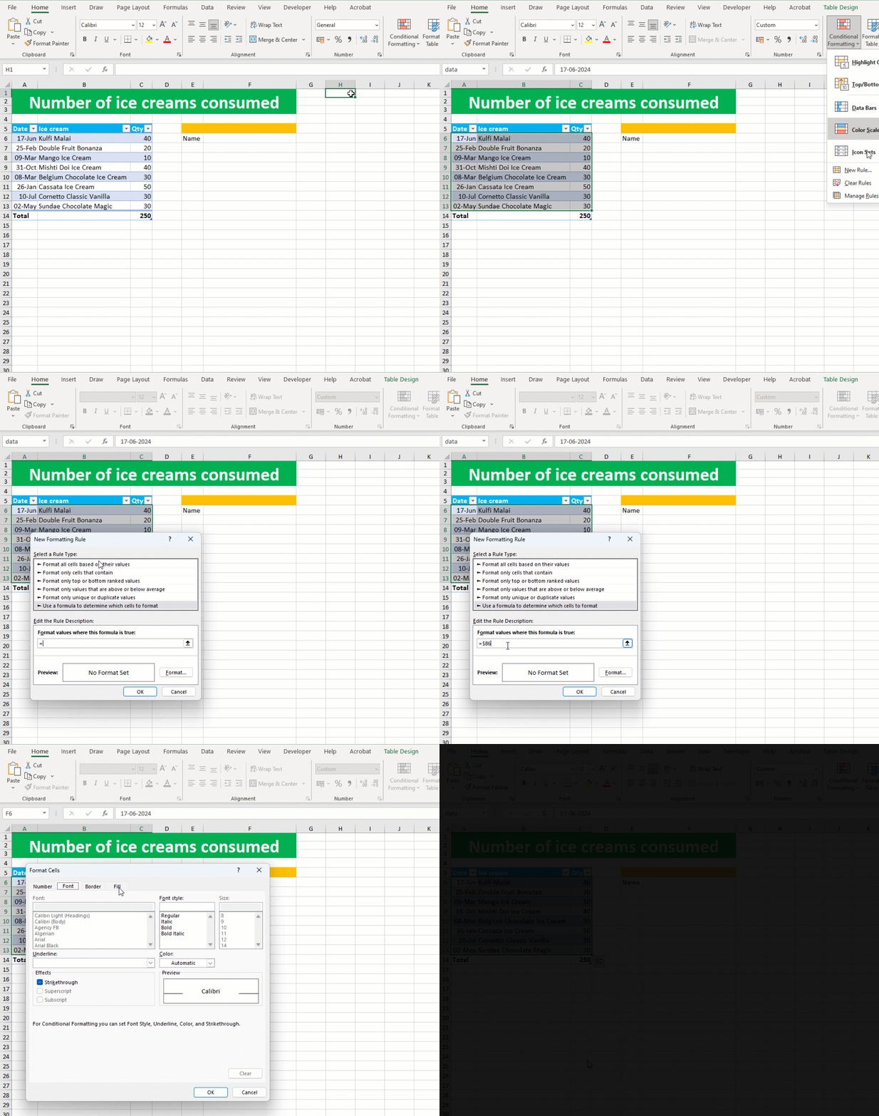
Highlight the source data (excluding column headers and total row). Move to the Home tab. Click on the Conditional Formatting menu and select the New Rule option. This will open the New Formatting Rule dialog box. Select Use a formula to determine which cells to format. Type this formula =$B6=$F$6. Click on the Format button, move to the Fill tab and select the yellow color. Click OK and OK again, like shown below:
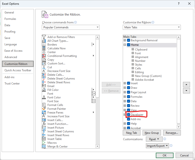
Now insert the required checkbox. To do so, go to File and choose Options. This will open the Excel Options dialog box. From the left pane, go to Customize Ribbon. Tick the Developer option. Click OK, like shown below. This will enable the Developer tab on the ribbon.
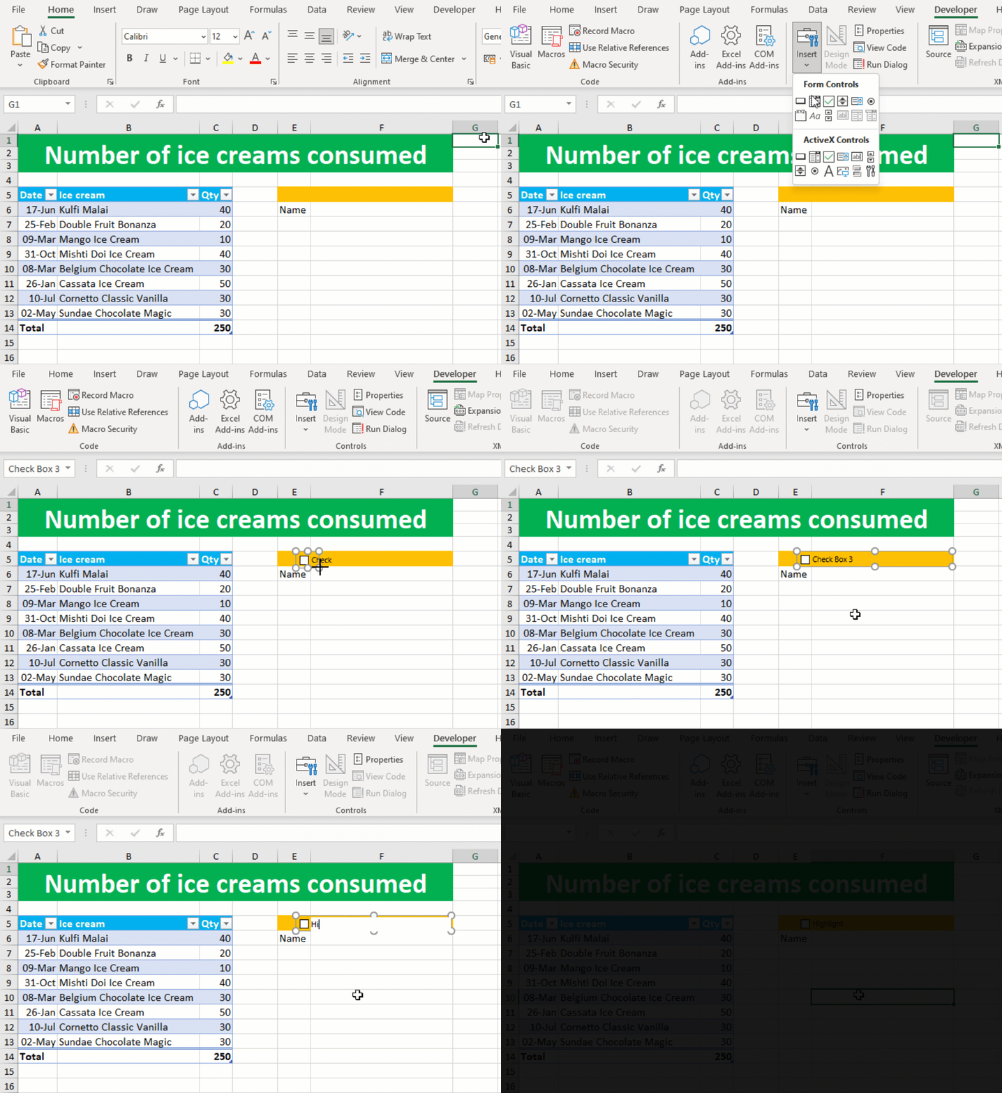
Move to the Developer tab on the ribbon. From the Controls group of the tab, click on the Insert menu and choose the check box control. Use the mouse to draw the check box onto the required place on the worksheet. Double-click on the text of the checkbox to edit the text, like shown below:
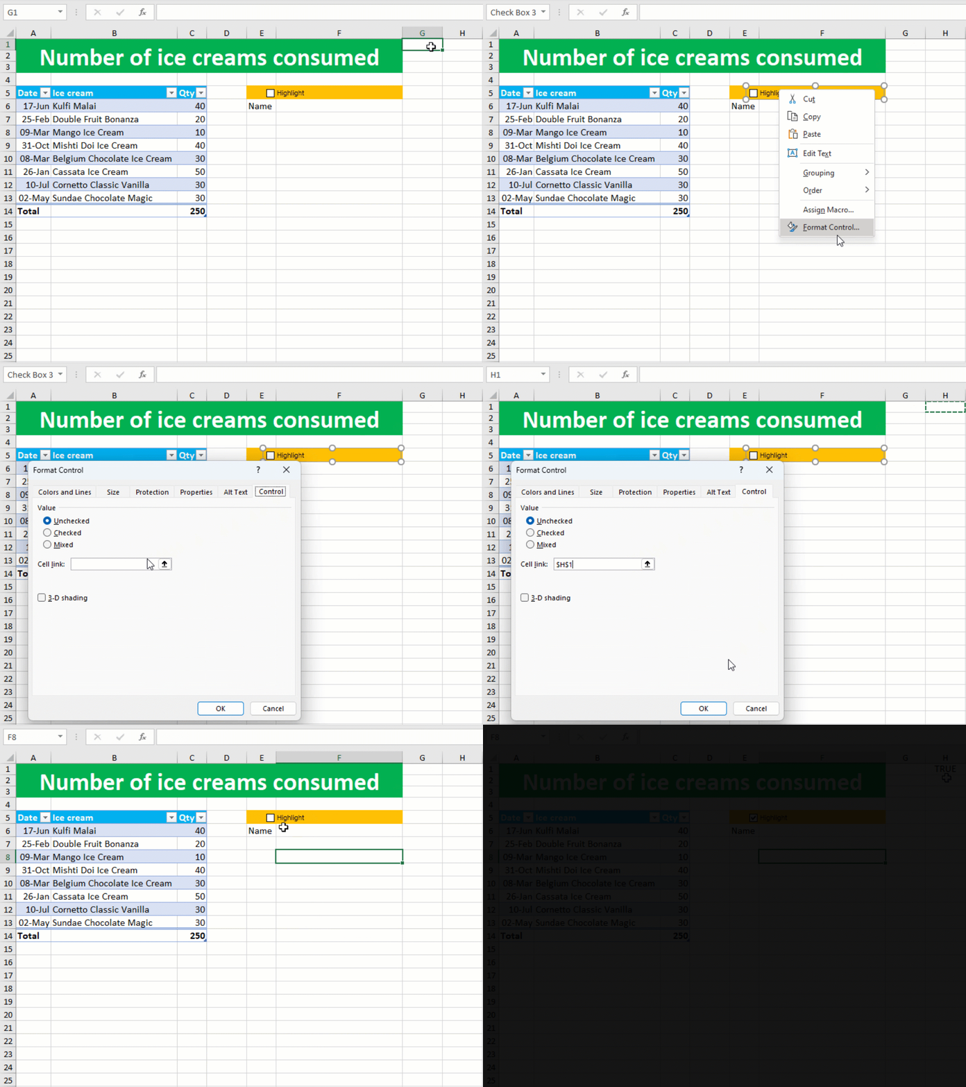
Right-click on the checkbox and select Format Control. Click on the Cell link field. Click on the H1 cell and click OK. Tick the Highlight checkbox. The TRUE value will appear on H1, like shown below:
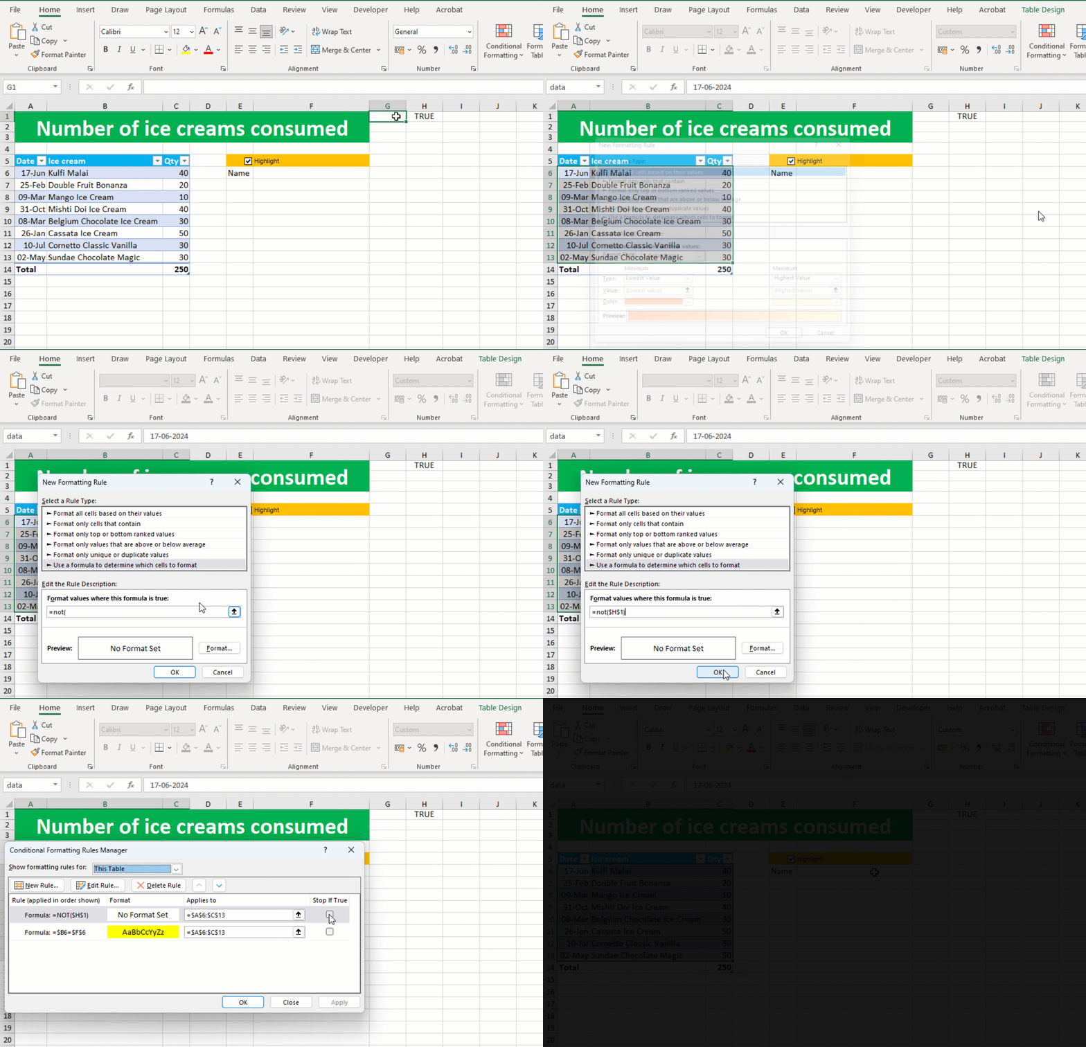
You need to apply one more formatting rule to the source data using the NOT function, like shown below:
As soon as you enter a new record in the source data, your dropdown list will update automatically. So, your dropdown is dynamic, like shown below:
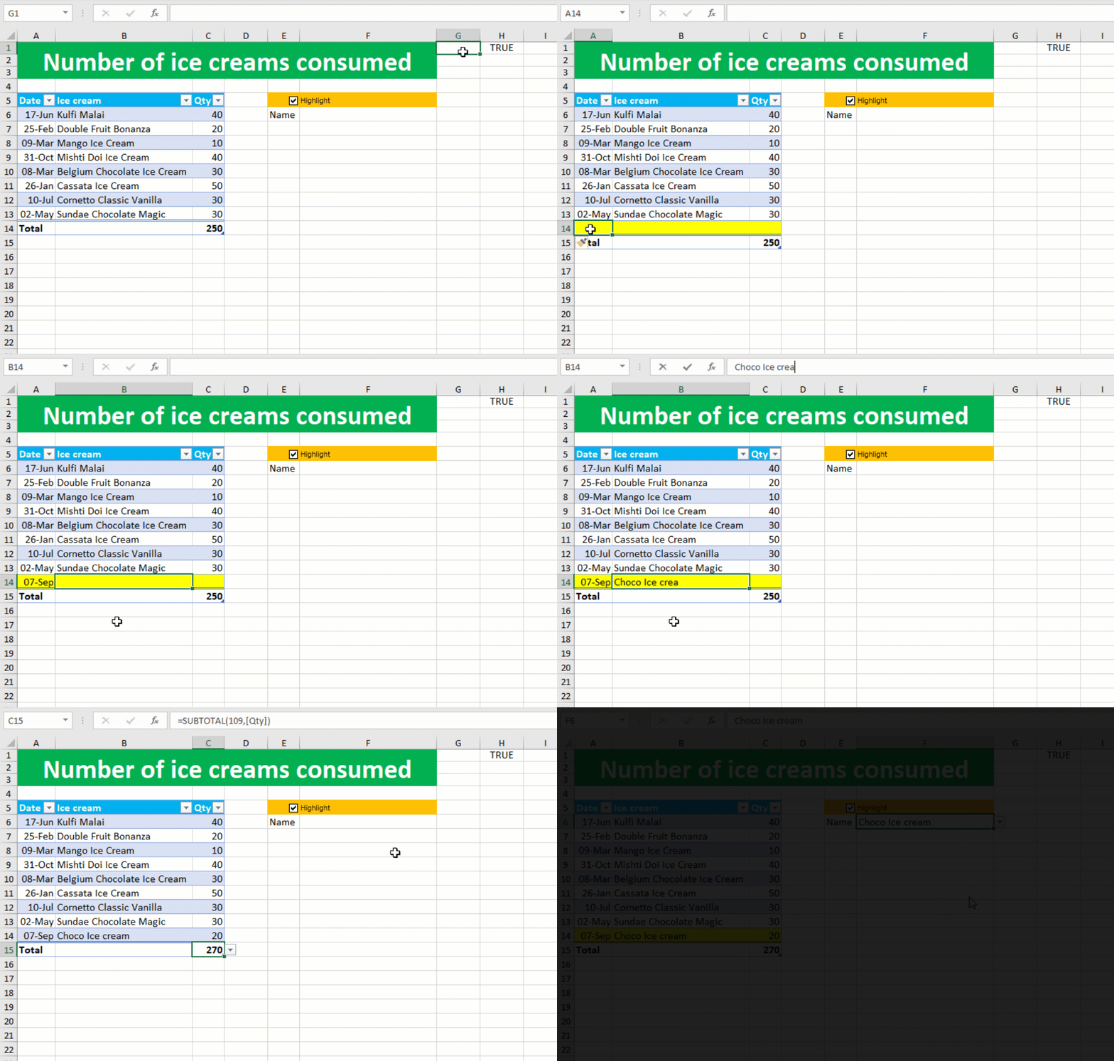
Your dropdown highlight using check box is ready! I hope this post helped you.

