In Excel, to lookup values from right to left, use the VLOOKUP function with the CHOOSE function. Here, I will use an Excel table, data validation to create dynamic dropdown and VLOOKUP - CHOOSE formula.
VLOOKUP looks for the value in the vertical data and returns a value from the given column number. CHOOSE returns the value at the given position.
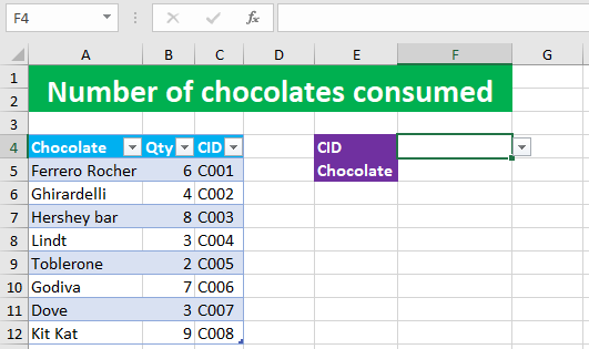
The following dataset contains the number of chocolates consumed:

Now I want the program to instantly return the chocolate name in F5 from column A based on the CID selection from the dropdown list in F4. To accomplish the task, I perform the following steps:
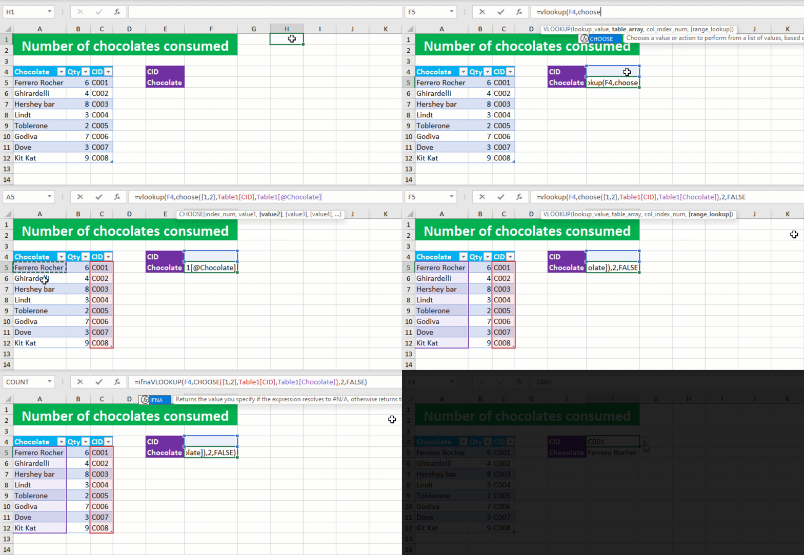
I convert the source data to an Excel table. I do so by clicking on a cell in the source data > Insert > Table > OK. By creating an Excel table, I can create a dynamic dropdown list.
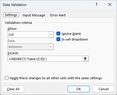
I use data validation to create a dynamic dropdown list in F4, listing all the CIDs in column C, by going to Data > Data Validation > List > =INDIRECT("Table1[CID]")

After all this, I construct my VLOOKUP - CHOOSE formula in F5, like shown below:

To replace the N/A error with an empty string "", I nest my entire formula in the IFNA function.
Your dropdown reverse Excel VLOOKUP is ready! I hope this post helped you.


