Here, we will learn how to filter and exclude columns using the Excel SORT, TAKE and CHOOSECOLS functions in one formula.
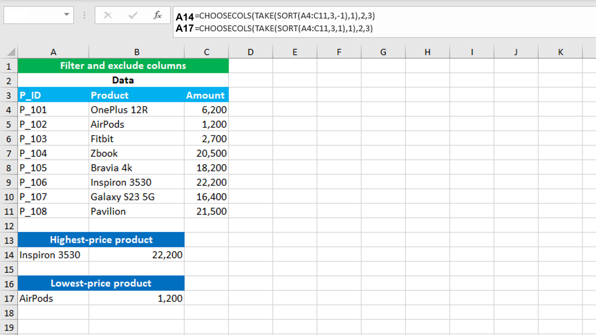
The dataset (shown in the image) contains a list of product names, their IDs and their prices. The goal is to use a single formula to extract the highest and the lowest-price product, while excluding the ID column . To accomplish the task, we create the header columns "Highest-price product" and "Lowest-price product" in the cells A13 and A16 respectively. A single formula based on the SORT, TAKE and CHOOSECOLS functions is used for both the tasks.
To extract the highest-price product and its amount, the formula in A14, is:
=CHOOSECOLS(TAKE(SORT(A4:C11,3,-1),1),2,3)
How this formula works
SORT is configured to sort the range A4:C11 by the third column "Amount" in descending order, like so: SORT(A4:C11,3,-1). SORT returns the sorted range to TAKE, which is configured to extract the first row, like so: TAKE(SORT(...),1). TAKE hands over the first row to CHOOSECOLS and this function is configured to return the second and third column, like this: CHOOSECOLS(TAKE(SORT(...),2,3). Therefore, we get the highest-price product name and its amount.
To extract the lowest-price product and its amount, the formula in A17, is:
=CHOOSECOLS(TAKE(SORT(A4:C11,3,1),1),2,3)
How this formula works
The formula is same as the previous one. The only difference is the SORT formula. This time SORT is configured to sort the range A4:C11 by the third column "Amount" in ascending order, like so: SORT(A4:C11,3,1). Therefore, we get the lowest-price product name and its amount.
You have successfully learnt how to filter and exclude columns using the Excel SORT, TAKE and CHOOSECOLS functions in one formula! I hope this post helped you.


