In Excel, to highlight top & bottom values and return their sum separately, I will use conditional formatting and use the SUM function, the LARGE function and the SMALL function.
The SUM function sums up the numbers, the LARGE function returns the nth largest numeric value and the SMALL function returns the nth smallest numeric value.
The following dataset contains the number of foods consumed:
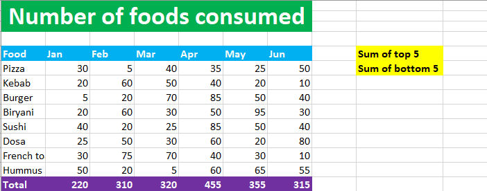
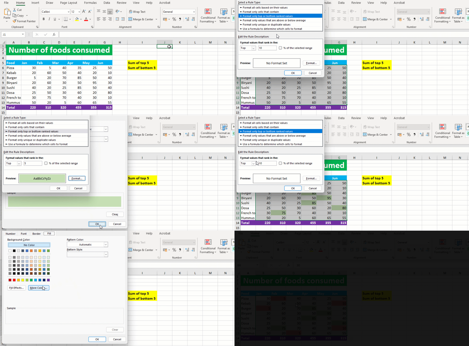
Now I want to highlight the top values with green color and bottom values with pink color and sum top 5 values and bottom 5 values.
To highlight the values, I create a new rule "Format only top or bottom ranked values" using conditional formatting, like shown below:
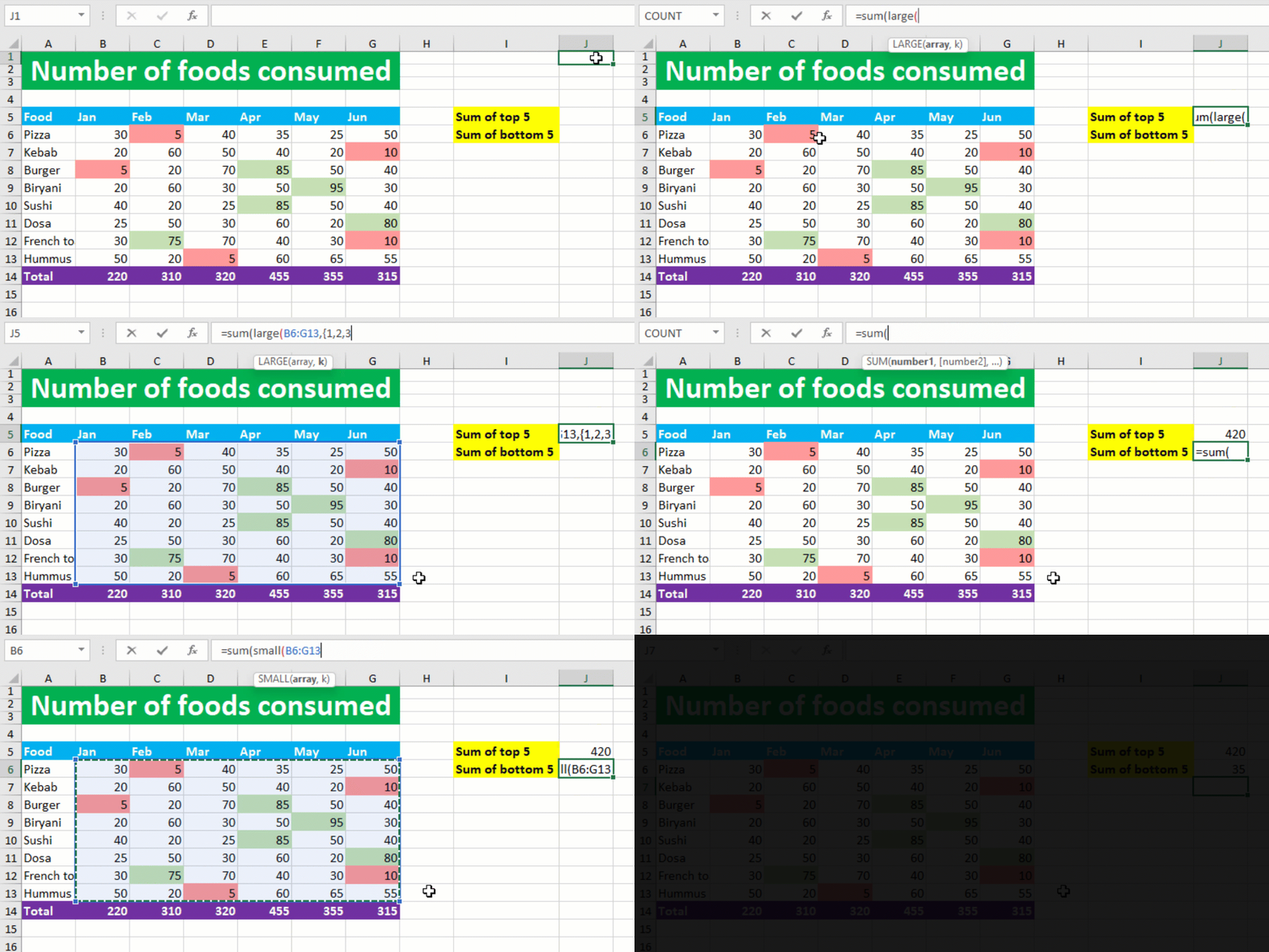
After this, I SUM up the top & bottom values using LARGE & SMALL functions in J5 and J6 respectively:
You have successfully accomplished the task! I hope this post helped you.

