Here, we will learn how to use the Excel logical functions: IFERROR and IFNA. Later, we will also learn how to use IFS VLOOKUP with IFERROR and IFNA.
IFERROR function
The Excel IFERROR function traps an Excel error and returns the given custom message, when a formula generates an error. When the formula does not generate an error, IFERROR does nothing. IFERROR traps the following Excel errors: #N/A, #VALUE!, #REF!, #DIV/0!, #NUM!, #NAME?, #NULL!, #CALC!, or #SPILL!.
IFERROR takes two arguments: value, value_if_error, all of which are required. The first argument value will take the value, reference or a formula to check for an error. The second argument value_if_error will take the custom message to return if the function traps an error.
Let's take a basic example. If we divide the number 2 by 0 (zero), Excel will throw the #DIV/0! error as division by zero is not possible. To replace the error with the custom message like "Division not possible", use IFERROR like this: =IFERROR(2/0,"Division not possible").
IFNA function
The Excel IFNA function traps the Excel #N/A error and returns the given custom message, when a formula generates the #N/A error. When the formula does not generate the error, IFNA does nothing.
IFNA takes two arguments: value, value_if_na, all of which are required. The first argument value will take the value, reference or a formula to check for the #N/A error. The second argument value_if_na will take the custom message to return if the function traps the #N/A error. For example, to replace the #N/A error with the custom message "Not applicable", use IFNA like this: =IFNA(#N/A,"Not applicable").
IFS VLOOKUP with IFERROR and IFNA
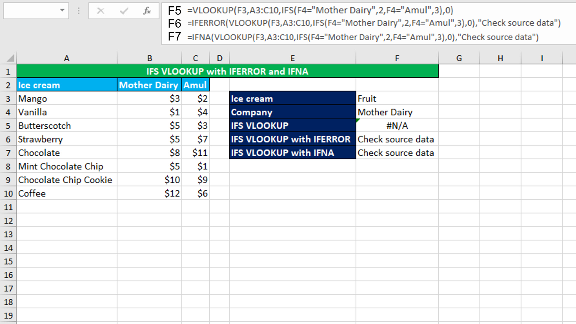
IFS can be used with VLOOKUP to return a corresponding value from the right column. We have a dataset (shown in image) that contains prices of ice creams by two companies in two separate columns. The goal is to get the price of "Fruit" ice cream of the company Mother Dairy using the IFS VLOOKUP formula. The formula in F5, is:
=VLOOKUP(F3,A3:C10,IFS(F4="Mother Dairy",2,F4="Amul",3),0)
The formula throws the N/A error since the lookup value "Fruit" is not there in the first column of the table array A3:C10. To replace the error with the custom message "Check source data", nest the entire formula in the IFERROR function. The formula in F6, is:
=IFERROR(VLOOKUP(F3,A3:C10,IFS(F4="Mother Dairy",2,F4="Amul",3),0),"Check source data")
Note that IFERROR traps any kind of Excel error. If you misspell a function's name, IFERROR will trap the #NAME? error and it would become difficult to solve the issue. In such a case, it becomes more sense to use the IFNA function that traps only the #N/A error. The formula in F7, is:
=IFNA(VLOOKUP(F3,A3:C10,IFS(F4="Mother Dairy",2,F4="Amul",3),0),"Check source data")
You have successfully learnt how to use the Excel logical functions: IFERROR and IFNA, and how to use IFS VLOOKUP with IFERROR and IFNA! I hope this post helped you.