The Excel IFS function tests the multiple conditions and returns a value corresponding to the first TRUE condition. The Excel IFNA function traps the N/A error and replaces the error with the custom value or message. The Excel IFERROR function, on the other hand, traps all the errors.
IFS function
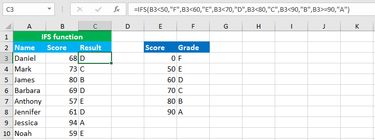
Below is the simple IFS formula that reads "return F if B3 is less than 50, E if B3 is less than 60, D, if B3 is less than 70, C, if B3 is less than 80, B, if B3 is less than 90 or A, if B3 is greater than or equals to 90":
=IFS(B3<50,"F",B3<60,"E",B3<70,"D",B3<80,"C",B3<90,"B",B3>=90,"A")
IFNA function
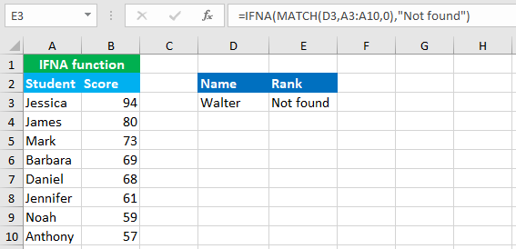
The IFNA function is commonly used with VLOOKUP and MATCH formulas. Below, I use the MATCH formula to return the numeric position of the student in D3 in the range A3:A10. Since the name "Walter" is not there in the range A3:A10, the formula returns the N/A error. To replace the error with the custom message "Not found", I nest the MATCH formula in the IFNA function, like so:
=IFNA(MATCH(D3,A3:A10,0),"Not found")
The difference between SWITCH and IFS is that SWITCH does not allows us to use logical operators like greater than (>), less than (<) and equals to (=), and therefore, must be an exact value match. On the other hand, IFS allows the use of logical operators.
IFERROR function
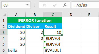
The IFERROR function can trap any type of Excel error and replaces it with the custom value or message. Below, we divide the numbers in two columns. The first formula returns the valid result. The next two formulas throw the DIV/0! error since we divide the number by zero and blank cell respectively. Last one returns the VALUE! error as the cell contains a text value.
IFS and VLOOKUP
IFS can be used with VLOOKUP to return a corresponding value from the right column. Below, we have a dataset that contains prices of ice creams by two companies in two separate columns. Now I want to get the price of mango ice cream of the company Mother Dairy, like shown below:
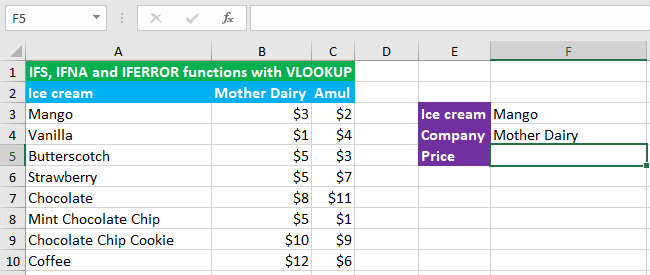
So, I construct the following formula in F5:
=VLOOKUP(F3,A3:C10,IFS(F4="Mother Dairy",2,F4="Amul",3),0)

IFS and IFNA VLOOKUP
When I change the lookup value to "Fruit", the same formula below throws the N/A error since the lookup value is not there in the first column of the table array A3:C10:
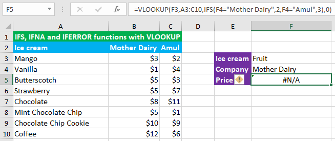
To replace the error with the empty string "", I nest the entire formula in the IFERROR function, like so:
=IFERROR(VLOOKUP(F3,A3:C10,IFS(F4="Mother Dairy",2,F4="Amul",3),0),"")
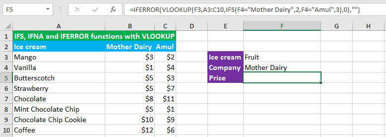
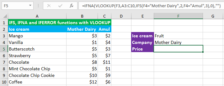
Using IFNA with VLOOKUP is more meaningful as IFNA traps only the N/A error. So, instead of using IFERROR, you can also use IFNA with VLOOKUP, like so:
=IFNA(VLOOKUP(F3,A3:C10,IFS(F4="Mother Dairy",2,F4="Amul",3),0),"")
You have successfully learnt about the Excel IFS, IFNA and IFERROR functions and how to use them with VLOOKUP! I hope this post helped you.


