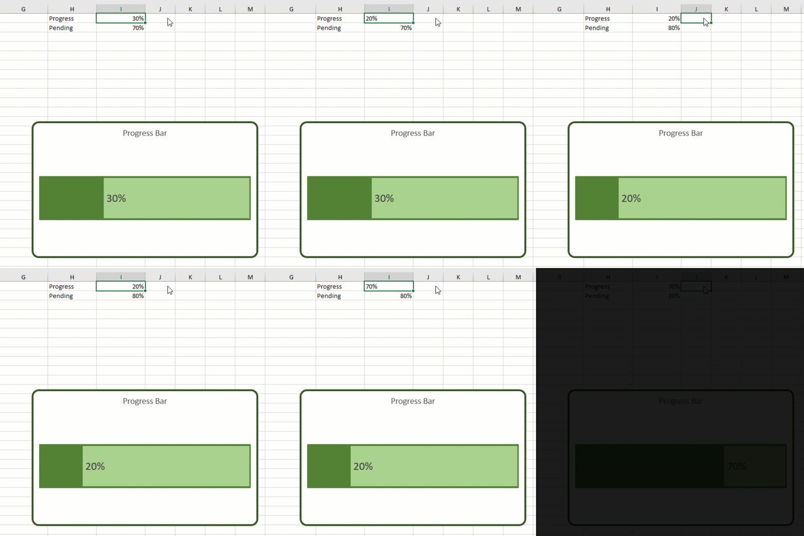
In Excel, to create a professional progress bar chart, I will use a bar chart and some formatting.
After performing the required steps to accomplish the task, you will be able to make a progress bar chart, like shown below:
In H1 and H2, I enter the words Progress and Pending respectively. In I1, I enter the progress percentage as 30%. To calculate the pending percentage, I enter this formula in I2: =100%-I1, like shown below:

Make sure the active cell is I2. Go to Insert > See All Charts arrow at the lower-right corner of the Charts group, like shown below:

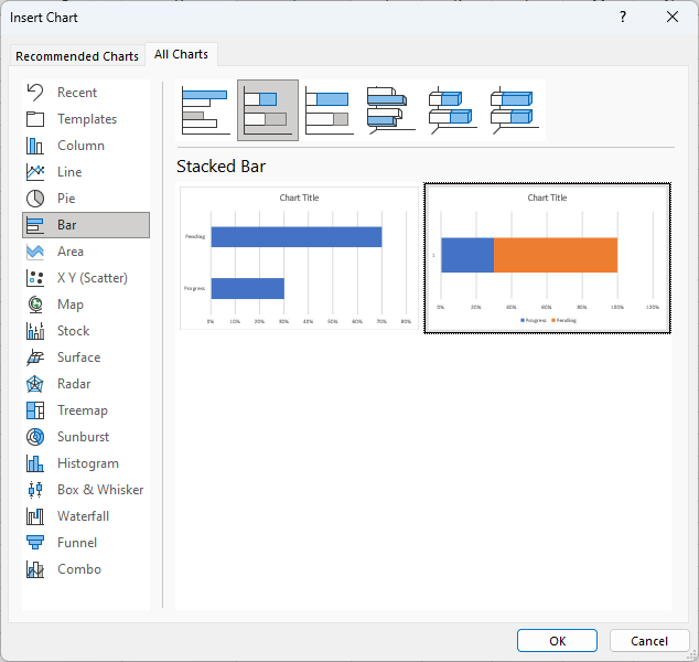
This will open the Insert Chart dialog box. Go to the All Charts tab. On the left pane, select Bar. Select the Stacked Bar (second) option from the list. Then, select the second Stacked Bar, like shown below:
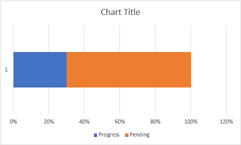
Press OK and this will insert the chart onto the worksheet:
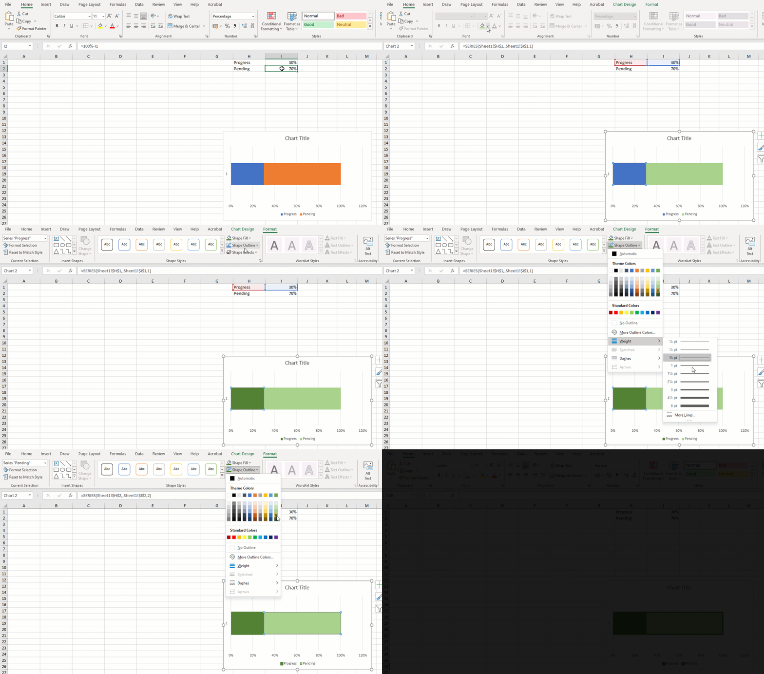
Customize the bars like shown below:
- Select the second bar > fill it with light green color.
- Select the first bar > fill it with dark green color.
- Select the first bar > Format > Shape Outline > dark green color > Shape Outline > Weight > 3 pt.
- Select the second bar > Format > Shape Outline > dark green color > Shape Outline > Weight > 3 pt.
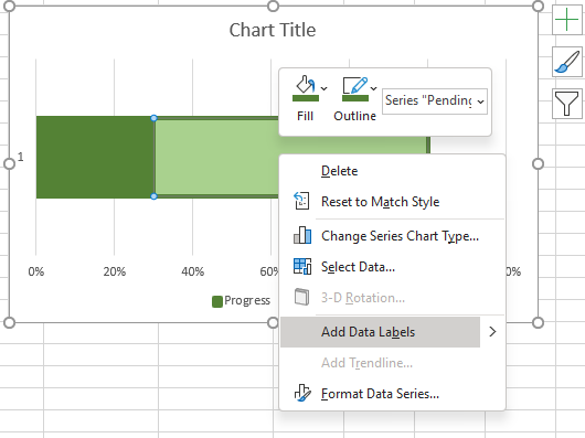
Right-click on the second bar and select the Add Data Labels option:
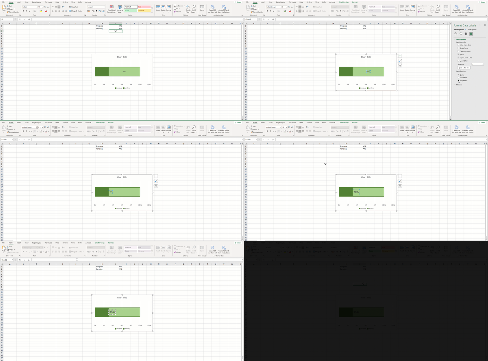
Format the data label, like shown below:
- Right-click on the data label > select Format Data Labels > Inside Base.
- Increase size of the label.
- Double-click on the label > Click on the formula bar > type equals sign = > Click on I1 > press Enter.
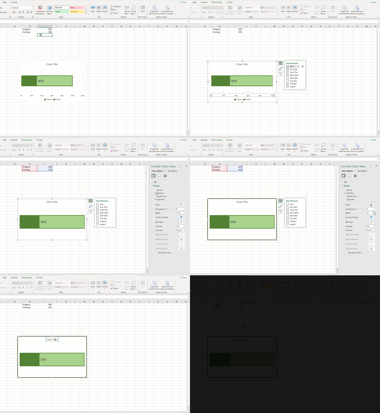
Do some more formatting to the chart area like shown below:
- Right click on the Axis on the Chart > Select Format Axis > Bounds > Maximum > 1.
- Click on the Plus icon > Untick Axes, Gridlines and Legend.
- Right-click on the chart area > Select Format Chart Area > Select Border > Solid line > Color: Dark green color > Width: 3 pt > tick Rounded corners.
- Click on the Chart Title > Enter the text Progress Bar.
Your professional progress bar chart is ready! I hope this post helped you.


