Here, we will learn how to use the Excel dynamic array function: SORTBY. Later, we will also learn how to reverse the table using SORTBY and the COLUMN function, that returns the column number for the reference.
SORTBY function
The Excel SORTBY function sorts the values of a range based on the values from another range.
SORTBY takes three arguments: array, by_array and sort_order. The first required argument array, will take the range which is to be sorted. The second required argument by_array, will take the values to be used for sorting. The third optional argument sort_order determines the sort direction. 1 will sort in ascending order and -1 will sort in descending order. By default, the function will sort in ascending order.
Reversing table using SORTBY and COLUMN
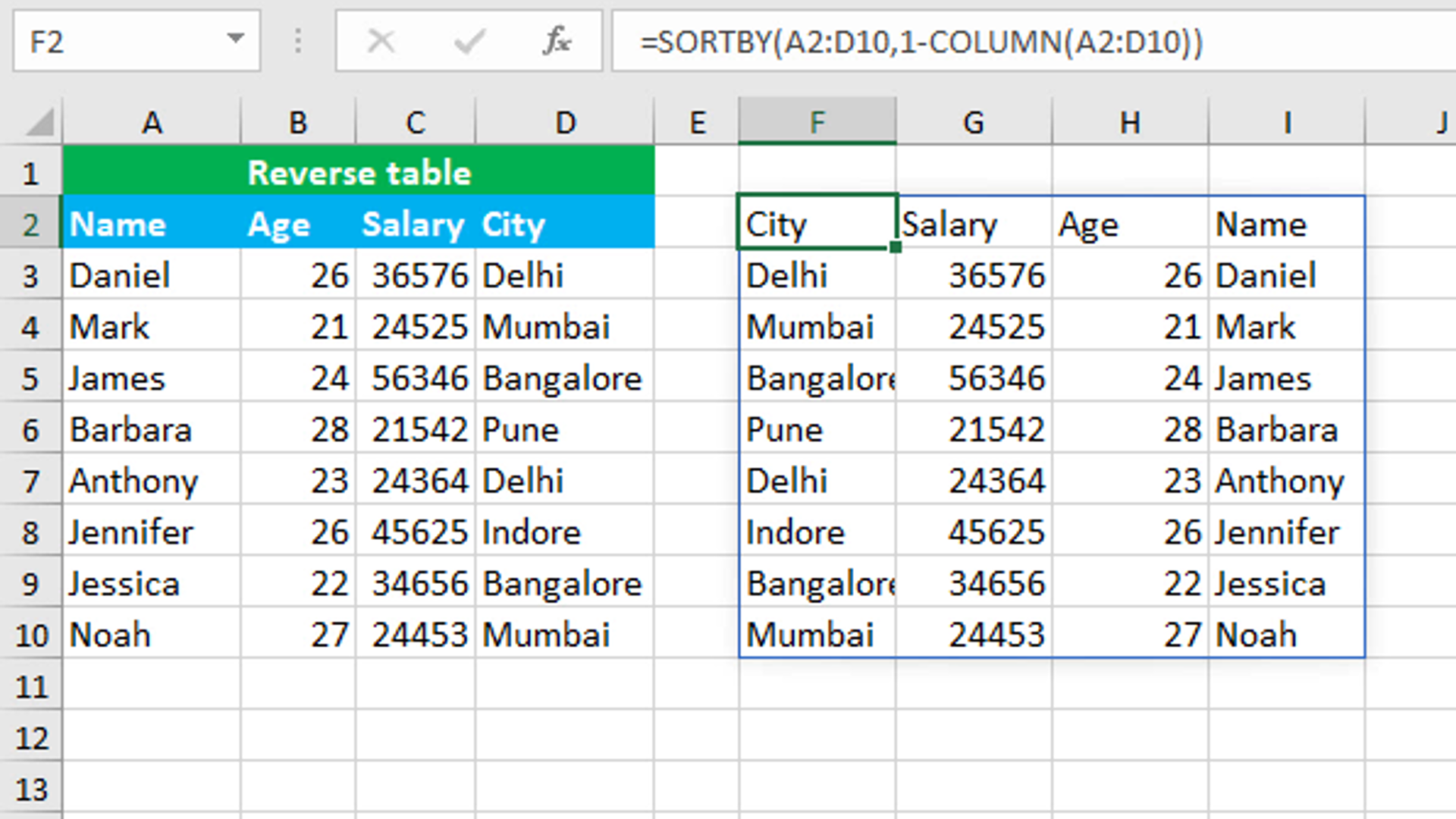
To reverse the table, use the SORTBY formula and nest the COLUMN function in the by_array argument. The formula in F2 is:
=SORTBY(A2:D10,1-COLUMN(A2:D10))
As soon as I press Enter, the formula spills the results into the multiple cells automatically in the range F2:I10.
How this formula works
Since COLUMN is given the range A2:D10, it returns the column numbers in an array, like: {1,2,3,4}. Each number in the array is subtracted from 1 and now the array becomes like: {0,-1,-2,-3}. Negative numbers in the array force the SORTBY formula to reverse the range A2:D10.
You have successfully learnt how to use the Excel dynamic array function: SORTBY, and how to reverse the table! I hope this post helped you.