Here, we will learn how to use the Excel text function: SUBSTITUTE. Later, we will also learn how to sum cells with text and numbers using SUM with the SUBSTITUTE function.
SUBSTITUTE function
The Excel SUBSTITUTE function replaces text in the given string by matching. For example, =SUBSTITUTE("abc&def&ghi","&","") returns the string "abcdefghi"; the character (&) is stripped. The function always returns the result in the text format even if the return value is a numeric value.
SUBSTITUTE takes four arguments: text, old_text, new_text, [instance_num]. The first required argument text will take the text to change. User can enter the value directly in the formula enclosing it with the double quotes (""), or a cell reference containing the value to change. The second required argument old_text will take the text we want to replace. The third required argument new_text will take the text we want to replace the old_text with. The final argument instance_num is optional, that specifies which occurrence of old_text we want to replace with new_text. The value must be entered as a numeric value else, #VALUE! error will be returned. By default, all instances are replaced. For example, =SUBSTITUTE("abc&def&ghi","&","",2) will return the string "abc&defghi"; the second occurrence of the character (&) is stripped.
Summing cells with text and numbers using SUM with SUBSTITUTE
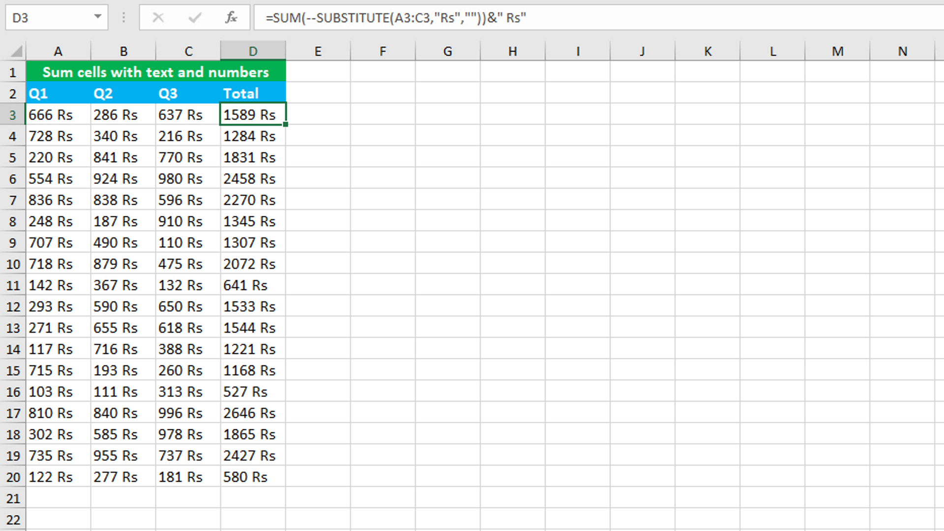
To sum cells with text and numbers, use the SUBSTITUTE formula and supply it to the SUM function, that sums up the numbers. My goal is to sum up the numbers in columns A, B and C and return the result in column D. Using SUM alone will not give the desired result as the values in column A, B and C contain both text and numeric values and SUM ignores the text values. So, if we will try to sum up the values in the range A3:C3, SUM will return zero. Therefore, we need to use SUM with SUBSTITUTE to strip the text " Rs". The formula in D3, copied down, is:
=SUM(--SUBSTITUTE(A3:C3,"Rs",""))&" Rs"
How this formula works
SUBSTITUTE strips the text value " Rs" from each numeric value in the range A3:C3. As said earlier, SUBSTITUTE returns the result in the text format so, SUBSTITUTE returns the numeric values in the text format. To convert those numeric text values into numeric values, insert the double negative operator (--) in front of the SUBSTITUTE formula. After this, supply the entire SUBSTITUTE formula to SUM that now sums up the numbers. SUM returns the result 1589. To join the numeric value 1589 with the text " Rs", use the ampersand (&) operator. Therefore, we get the final output "1589 Rs" in the text format.
You have successfully learnt how to use the Excel text function: SUBSTITUTE, and how to sum cells with text and numbers using SUM with the SUBSTITUTE function! I hope this post helped you.