Here, we will learn how to use the Excel dynamic array function: TOROW. Later, we will also learn how to sort and extract unique values into row using TOROW and the SORT and UNIQUE functions.
TOROW function
The Excel TOROW function transforms the given data into a single row, scanning values by row.
TOROW takes three arguments: array, [ignore], [scan_by_column]. The first required argument array will take the range to transform. The second optional argument ignore will control what values the function can ignore. Specifying 1 will ignore blanks; 2 will ignore errors and 3 will ignore both blanks and errors. Omitting the argument will take the default value of 0 (zero) that will keep all the values. The third optional argument scan_by_column will control how the function will scan the values, by row or column. Specifying TRUE will scan the values by column. Omitting the argument will take the default value of FALSE that will scan the values by row.
Basic examples
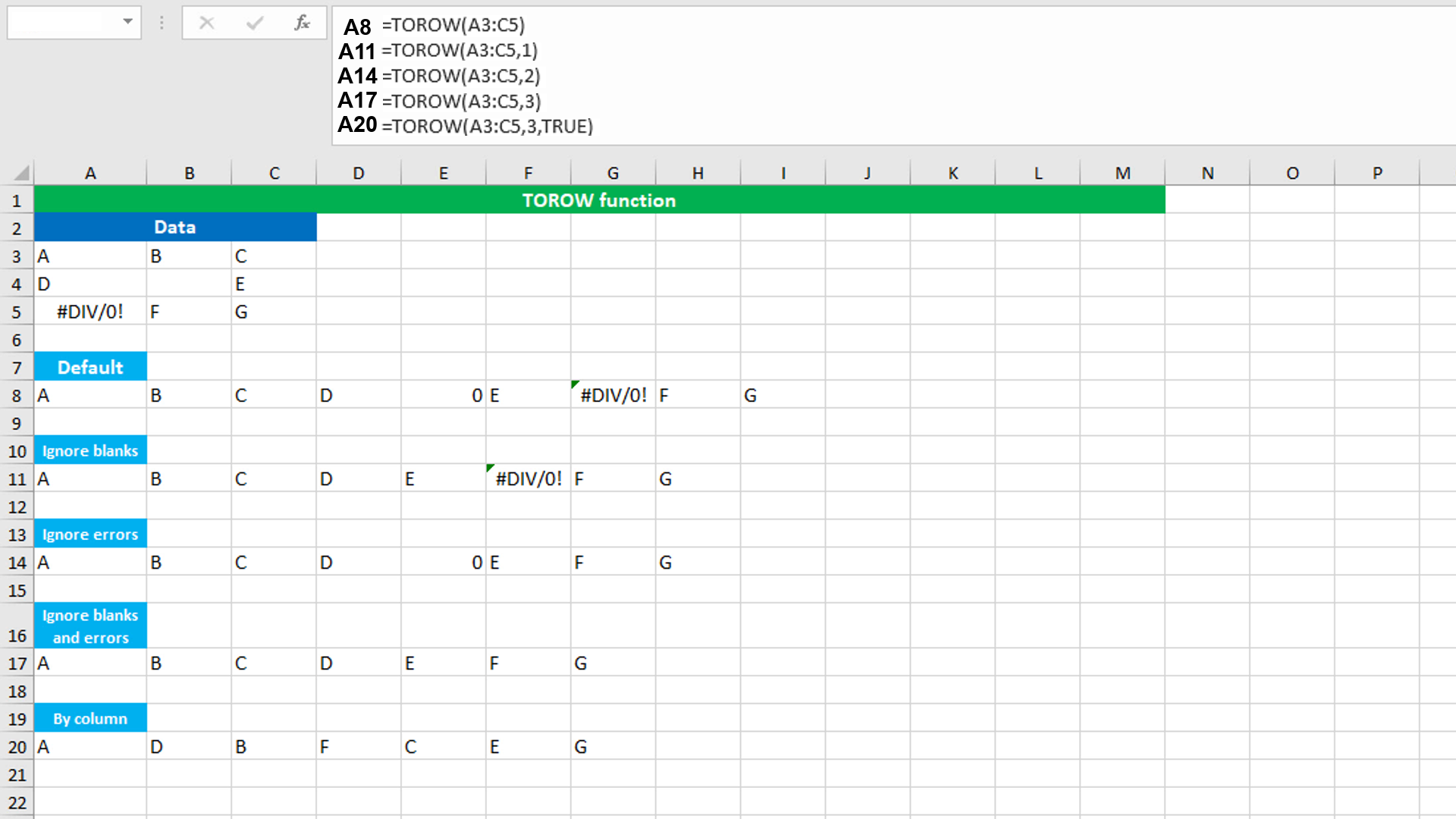
By default, TOROW will transform the given data into a single row, keeping all the values and scanning the values by row. The formula in A8 (in the image shown) is:
=TOROW(A3:C5)
To ignore blanks or/and errors, the following formulas are applied in A11, A14, A17 respectively:
=TOROW(A3:C5,1)
=TOROW(A3:C5,2)
=TOROW(A3:C5,3)
In A20, the function has been set to scan the values by column by specifying TRUE in the scan_by_column argument:
=TOROW(A3:C5,3,TRUE)
Sorting and extracting unique values into row using TOROW with SORT and UNIQUE
To transform a data into a single row and to sort and extract unique values from the same data, use a formula based on the TOROW, SORT and UNIQUE functions.
The dataset (shown in the image) contains a data in three non-adjacent ranges. The goal is to join these ranges, sort the data alphabetically and extract unique values.

The formula in A8 is:
=UNIQUE(SORT(TOROW((A3:B5,D3:E5,G3:H5)),,,TRUE),TRUE)
How this formula works
TOROW joins the given three non-adjacent ranges (A3:B5,D3:E5,G3:H5) and transforms them into a single row. This result goes to SORT that is configured to sort the row range alphabetically and horizontally (by column), like this: SORT(TOROW((...)),,,TRUE). Finally, SORT hands over the result to UNIQUE that is configured to return unique values horizontally (by column), like this: UNIQUE((TOROW((...)),,,),TRUE)
You have successfully learnt how to use the Excel dynamic array function: TOROW, and how to sort and extract unique values into row using TOROW and the SORT and UNIQUE functions! I hope this post helped you.